
A random forest combines many decision trees to produce a more stable prediction than a single tree. The method works well on tabular classification and regression problems, but its defaults can consume too much memory and its feature importances are easy to misread. Here is the mechanism, the parameters that matter, and a reliable scikit-learn workflow.
What is a random forest?
A random forest is a supervised machine learning algorithm that combines many decision trees. Each tree sees a different sample of the training rows, and each split considers a random subset of the features. The forest aggregates the trees' predictions to reduce the instability of any one tree.
The standard algorithm handles two tasks:
| Task | Each tree produces | The forest produces |
|---|---|---|
| Classification | A probability for each class | Mean class probabilities, then the class with the highest mean probability |
| Regression | A numeric prediction | The mean of the trees' predictions |
That classification detail matters. In scikit-learn, RandomForestClassifier averages the trees' class probabilities. It does not simply count one hard vote per tree. A tree's probability is the share of training samples from each class in the reached leaf, as the classifier documentation specifies.
Random forest is an ensemble method, not a deep learning model. Leo Breiman's 2001 random forest paper formalized the algorithm and tied its generalization error to two properties: the strength of the individual trees and the correlation between them. Stronger trees help, while highly correlated trees make fewer independent errors for averaging to cancel.
Our ensemble learning guide explains how that principle also appears in bagging, boosting, voting, and stacking.
How the random forest algorithm works
Training a forest follows five steps.
- Draw a bootstrap sample. Sample
nrows with replacement from a training set containingnrows. Some rows appear more than once, while others are absent. - Grow a decision tree. At each node, randomly select
max_featurescandidate columns. Find the best split among those candidates using the chosen impurity criterion. - Repeat for many trees. Each tree receives a new bootstrap sample and new feature candidates at every split.
- Aggregate the predictions. Average numeric outputs for regression or class probabilities for classification.
- Evaluate on unseen data. Use cross-validation, a validation set, or out-of-bag predictions during development. Keep a final test set untouched until model selection is complete.
The two sources of randomness solve different problems. Bootstrap sampling changes the training rows. Feature sampling reduces the chance that the same dominant feature drives every tree. The resulting trees make less correlated errors, so averaging reduces variance.
max_features applies at every split
max_features is often misunderstood. It usually limits the candidates examined at one node, not the total features available to an entire tree.
Suppose a dataset has 25 input features and max_features="sqrt". Each node considers about five randomly selected features, chooses the best split among them, and then passes different row subsets to its children. The next node draws another random feature subset. One finished tree may use far more than five features across all its nodes.
Lower values create more varied trees, but each tree has fewer candidate splits. Higher values can strengthen individual trees while also making them more similar. This strength-correlation tradeoff is why max_features deserves validation rather than a universal prescription.
Out-of-bag samples provide a built-in estimate
Sampling n times with replacement does not place every training row in a tree's bootstrap sample. For one row, the probability of being left out is:
(1 - 1/n)^n ≈ e^-1 ≈ 0.368
About 36.8% of the rows are therefore out of bag for a given tree when the sample is large. The forest can predict each training row using only trees that did not train on it. This produces an out-of-bag (OOB) score without fitting a separate validation forest.
OOB scoring is useful for fast iteration and for plotting error against the number of trees. It does not replace a test set. It also assumes that row-wise resampling matches the deployment problem. Time series, repeated users, patients, accounts, and other grouped data need time-aware or group-aware validation.
A random forest classification example in Python
This scikit-learn example trains a classifier on the built-in breast cancer dataset. It uses a stratified split, reports both accuracy and receiver operating characteristic area under the curve (ROC AUC), and enables OOB scoring.
from sklearn.datasets import load_breast_cancer
from sklearn.ensemble import RandomForestClassifier
from sklearn.metrics import accuracy_score, roc_auc_score
from sklearn.model_selection import train_test_split

X, y = load_breast_cancer(return_X_y=True, as_frame=True)

X_train, X_test, y_train, y_test = train_test_split(
    X,
    y,
    test_size=0.25,
    stratify=y,
    random_state=42,
)

model = RandomForestClassifier(
    n_estimators=300,
    max_features="sqrt",
    min_samples_leaf=2,
    class_weight="balanced",
    oob_score=True,
    n_jobs=-1,
    random_state=42,
)

model.fit(X_train, y_train)

predicted_class = model.predict(X_test)
positive_probability = model.predict_proba(X_test)[:, 1]

print("Accuracy:", accuracy_score(y_test, predicted_class))
print("ROC AUC:", roc_auc_score(y_test, positive_probability))
print("OOB accuracy:", model.oob_score_)
The three scores answer different questions. Accuracy evaluates hard class decisions at the model's current threshold. ROC AUC evaluates how well the probability scores rank positive examples above negative ones across thresholds. OOB accuracy is a development estimate based only on the training partition.
Choose metrics from the real cost of errors. For an imbalanced problem, inspect precision, recall, the precision-recall curve, and confusion matrices alongside accuracy. Our ROC AUC calculation guide shows what the metric measures and why threshold selection is a separate decision.
The random forest hyperparameters that matter
Scikit-learn exposes many parameters. Most tuning effort should go to a smaller set.
| Parameter | What it controls | Practical tuning signal |
|---|---|---|
n_estimators | Number of trees | Increase it until validation or OOB performance stabilizes. More trees continue to add training and inference cost. |
max_features | Candidate features at each split | Lower values increase tree diversity. Higher values give each node more possible splits. |
max_depth | Maximum depth per tree | Limit it when unconstrained trees overfit, become slow, or consume too much memory. |
min_samples_leaf | Minimum rows in a leaf | Larger leaves smooth predictions and often help noisy data or probability estimates. |
min_samples_split | Minimum rows needed to split a node | Larger values suppress splits supported by few observations. |
max_samples | Rows drawn for each tree | Smaller bootstrap samples reduce cost and can increase diversity. |
class_weight | Relative class weights | Use it when the training objective should penalize minority-class errors more heavily. Evaluate the resulting threshold and probabilities. |
criterion | Split-quality measure | Usually a lower-priority choice than tree size, feature sampling, and the evaluation design. |
The current RandomForestClassifier API defaults to n_estimators=100, max_features="sqrt", and bootstrap=True. The current RandomForestRegressor API also defaults to n_estimators=100 and bootstrap=True, while its max_features=1.0 considers all features at a split. Treat these defaults as starting points. Dataset size, feature redundancy, noise, and latency requirements determine the useful settings.
Two other parameters affect operation rather than model capacity:
n_jobs=-1uses all available processors for parallel work. Set an explicit job count in shared environments where the process must not claim every core.random_statemakes the sampling reproducible. Reproducibility helps compare experiments, but one seed does not measure uncertainty. Re-run finalists across several seeds when the dataset is small or results are close.
Scikit-learn's unconstrained defaults grow fully developed trees, which can be large. Measure serialized model size, peak memory, batch throughput, and single-row latency before declaring a configuration ready.
A tuning workflow that avoids leakage
Hyperparameter search cannot repair a weak validation design. Use this order:
- Define the prediction unit and horizon. Decide what one row represents and when its features would be available in production.
- Create the splits first. Use stratification for ordinary classification, group splits for repeated entities, and chronological splits when the model predicts the future.
- Build simple baselines. Compare the forest with a dummy predictor and an appropriate linear or single-tree model.
- Choose the metric before tuning. Use a ranking metric such as ROC AUC when ranking quality matters. Also measure performance at the intended operating threshold with metrics that reflect the costs of false positives and false negatives. Include probability loss when probability quality matters. Include operational metrics when prediction cost matters.
- Raise
n_estimatorsuntil results stabilize. A stable tree count makes comparisons of other parameters less noisy. - Tune tree diversity and capacity. Search
max_features,min_samples_leaf,max_depth, and, when useful,max_samples. Randomized search usually covers wide numeric ranges more efficiently than a large Cartesian grid. - Lock the configuration and run the test once. Report the test result with relevant slices, uncertainty, model size, and latency.
Never fit preprocessing, feature selection, resampling, or target encoding on the complete dataset before cross-validation. Put learned transformations inside the validation pipeline so every fold learns them from its own training rows.
When random forest is a good choice
Random forests are a strong baseline for tabular data when:
- nonlinear effects and feature interactions are likely;
- a single decision tree is too unstable;
- you want useful performance without scaling numeric features;
- training can run in parallel across trees;
- the dataset is moderate enough for many trees to fit in memory; and
- prediction within the observed feature and target ranges is sufficient.
They also give you OOB predictions, partial dependence tools, and several feature-inspection methods. Those aids support debugging, but they do not make the model intrinsically causal or fully interpretable.
Where random forests fall short
A random forest is a poor default in several cases:
- Strict memory or latency limits: Hundreds of deep trees can create a large model and many branches to traverse per prediction.
- Regression that must extrapolate: A forest averages values stored in leaves. It cannot extend a linear trend beyond the target values represented in its training leaves.
- Very sparse, high-dimensional problems: Linear models can be faster and more accurate for tasks such as bag-of-words text classification.
- Raw images, audio, or long text: These inputs usually need learned representations or purpose-built models before a tree ensemble becomes useful.
- A simple relationship that must be explained directly: A small decision tree or regularized linear model may trade some predictive accuracy for much clearer behavior.
- Maximum tabular accuracy under a larger tuning budget: Gradient-boosted trees often deserve a head-to-head benchmark. They build trees sequentially, which changes their training behavior and operating tradeoffs.
| Model | Good fit | Main tradeoff |
|---|---|---|
| Decision tree | A compact rule set and visual explanation matter most | High variance and usually weaker predictive accuracy |
| Random forest | You want a dependable nonlinear baseline with parallel training | Larger model and less direct interpretation |
| Gradient-boosted trees | Predictive performance justifies more tuning and sequential training | Greater sensitivity to settings and a less parallel training process |
Treat feature importance as a diagnostic
feature_importances_ reports mean decrease in impurity across a forest. It is fast to compute, but scikit-learn warns that impurity-based importance can favor high-cardinality features, which offer more possible split points.
Permutation importance asks a different question: how much does a chosen score fall when one feature is shuffled? Compute it on validation or test-like data, not the same rows used to fit the model. Correlated features still complicate the result. If two columns contain similar information, shuffling one may have little effect because the other remains available.
Neither method proves that a feature causes the outcome. Use importance to form debugging questions, then inspect leakage, feature availability, correlated groups, partial dependence, and performance after removing or grouping suspect variables.
Classification probabilities need similar caution. Random forests can rank examples well while producing probabilities that need calibration. If a score drives pricing, routing, or a risk decision, evaluate reliability curves and probability losses. Our confidence calibration guide provides a production workflow.
Build the baseline, then test the tradeoffs
A reliable first experiment is simple: preserve a locked test set, fit enough trees for the validation curve to stabilize, and tune max_features with one or two tree-size controls. Compare the result with a linear baseline, a single tree, and a gradient-boosted model under the same splits and metrics.
Choose the model that meets the defined requirements for predictive quality, calibration, latency, memory, stability, and explainability. Keep the random forest only when its held-out results and operating measurements justify the extra model size and inference work over a simpler baseline.