

An ensemble (Multiple Classifier System) is an algorithm that consists of multiple machine learning algorithms, and the process of building an ensemble is called ensemble learning.
Voting & Average-Based Ensemble Methods Machine Learning
Two of the basic ensemble methods in machine learning are voting and averaging. Voting techniques are used in predictive classification problems, while average-based methods are a basis for regression.
Ensemble Averaging for Regression
The simplest example of an ensemble in regression is averaging several algorithms:
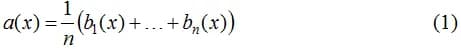
The algorithms that make up the ensemble (in (1) - bt) are called base learners. If we consider the values of the basic algorithms on the object as independent random variables with the same mean and the same final variance, then it is clear that the random variable (1) has the same expected value but lower variance:
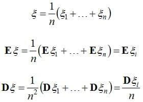
Note: the requirement that the expected value of the answers of the basic algorithms have to be equal is quite natural: if we take the algorithms from the unbiased model, then their mathematical expectations not only coincide, but are also equal to the value of the true label. But the requirement of equality of variances no longer has an acceptable justification, but to justify the effectiveness of the ensemble, one can require less ... the question is: what exactly?
Majority Voting Ensemble Machine Learning
In machine learning classification problems, the simplest example of an ensemble is a majority committee:

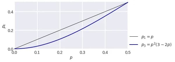
"mode" here is the value that occurs more often among the arguments of the function. If we consider the classification problem with two classes {0, 1} and three algorithms, each of which is wrong with probability p, then under the assumption that their answers are independent random variables, we get that the committee of most of these three algorithms is wrong with probability pp(3-2p). As seen in the figure below, this expression can be significantly less than p (for p=0.1 it’s nearly two times less), i.e. the use of such an ensemble reduces the error of the basic algorithms.
Note: if we consider a larger number of algorithms, then according to the Hoeffding's inequality, the error of the majority committee is as follows:
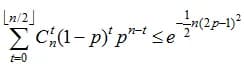
i.e. it decreases exponentially with an increase in the number of basic algorithms.
Note: our theoretical justification is not entirely suitable for a real practical situation, since the regressors / classifiers are not independent, so they:
- solve one problem,
- are adjusted to one target vector,
- can be from one ensemble model machine learning (or from several, but still in a small number).
Improving Performance and Accuracy with Diversity of Machine Learning Ensemble Methods
Most of the techniques in applied ensemble are aimed at making the ensemble "sufficiently diverse", then the errors of individual algorithms on individual objects will be compensated for by the correct operation of other algorithms. Basically, when building an ensemble you:
- improve the quality of basic algorithms,
- increase the diversity of the underlying algorithms.
As will be shown later, diversity is increased at the expense of (examples are indicated in parentheses where the corresponding technique is applied):
"Variation" of the training sample (Bagging (machine learning ensemble)),
"Variation" of features (Random Subspaces),
"Variation" of the target vector (Error-Correcting Output Codes (ECOC), deformation of the target feature),
"Varying" models (use of different models, stacking),
“Variation” in the model (use of different algorithms within one, randomization in the algorithm is a random forest).
Increasing Variance in Ensemble Models Machine Learning
Let’s take a look at the examples of natural (already implemented in the model) and artificial (manual) variation within the same model. When training neural networks, a lot can depend on the initial initialization of parameters, therefore, even when using the same architecture of a neural network, after two different training procedures, we can get different algorithms. Manual variation is achieved by forcibly fixing some parameters of the algorithm, for example, you can boost the decision trees of depth 1, 2, 3, etc., and then ensemble the resulting algorithms (they will be different, although formally we used the same model).
Another argument in favor of the variety of algorithms in the ensemble can be made using such an experiment. We will have a binary vector encoding the correct answers of the algorithm on the control sample in a problem with two classes: 1 - correct answer, 0 - error. If we construct several identical algorithms (at least in the sense that the indicated characteristic vectors of correct answers coincide), then voting on these algorithms will have exactly the same vector:
algorithm 1: 1111110000 quality = 0.6 algorithm 2: 1111110000 quality = 0.6 algorithm 3: 1111110000 quality = 0.6 ensemble : 1111110000 quality = 0.6
Now let's build similar algorithms:
algorithm 1: 1111110000 quality = 0.6 algorithm 2: 1111101000 quality = 0.6 algorithm 3: 1111100100 quality = 0.6 ensemble : 1111100000 quality = 0.5
And now let's build completely different algorithms:
algorithm 1: 1010010111 quality = 0.6 algorithm 2: 1100110011 quality = 0.6 algorithm 3: 1111110000 quality = 0.6 ensemble : 1110110011 quality = 0.7
As you can see, the ensemble of “very diverse” algorithms showed the best quality. The question is: is there a catch in this example?
In general, the ensemble is written out as follows:
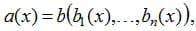
b here is some algorithm (i.e. function), which is commonly called a meta-estimator. As you can see, expressions (1) and (2) are a special case of this function.
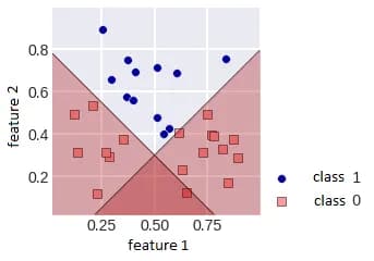
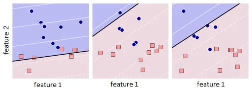
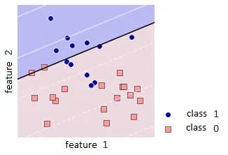
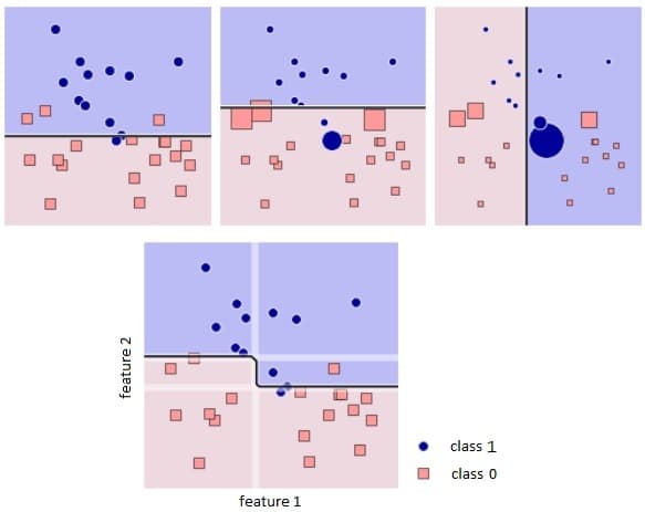
The rationale for using ensembles in machine learning is usually statistical - given above, when we estimated the ensemble error based on the probabilistic nature of the algorithms' responses; it can be computational, the ensemble parallelizes the process: we train several basic algorithms in parallel and the meta-estimator "combines" the received answers; representational - often an ensemble can represent a much more complex function than any basic algorithm. The latter can be illustrated by the figure below: a binary classification problem is shown, in which a linear algorithm cannot be tuned to 100% quality, but a simple ensemble of linear algorithms can. Thus, ensembles allow solving complex problems with simple models; the complication of the solution for the possibility of good tuning to the data occurs at the level of the meta-algorithm.
Boosting, Stacking, Bagging & Other Techniques for Setting up Robust Predictive Models
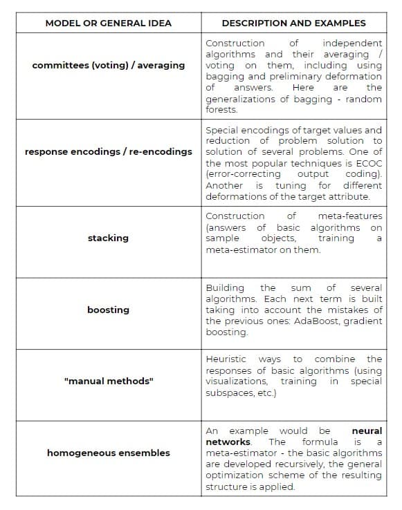
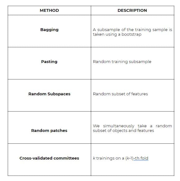
Now, let’s discuss the basic ensemble methods in machine learning for aggregating base ML models as summarized in the following table.
Committees (Voting Ensembles) / Averaging
We got acquainted with this simplest way of building ensembles in the examples above. Note that in the general case, any Cauchy distribution can be used. For example, in problems of detecting anomalies, the maximum can be used as a meta-classifier: each basic algorithm gives its own estimate of the probability that a particular object is an anomaly (not like a training sample), we rely on the maximum estimate. Since such tasks arise in areas where an anomaly cannot be missed (detection of breakdowns, hacker attacks, insiders on the exchange, etc.), they act according to the logic of "raise the alarm at the slightest suspicion."
Often, when using the Mean Absolute Error (MAE) function in a regression problem, the median of the basic algorithms shows a quality that is higher than the arithmetic mean. In problems of binary classification when using AUC ROC, it is often not the assessments of belonging to class 1 that are averaged, and the ranks are as follows:
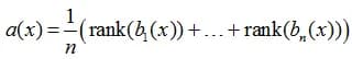
We can try to explain this by the fact that the “correct ordering” of objects in the binary classification problem is important for the AUC ROC functional, and not specific values of estimates. The rank function allows, to a lesser extent, to take into account the values themselves that the algorithms produce, and to a greater extent, the order on the objects of the control sample.
Weighted Averaging
Instead of the usual averaging / voting, weighted averaging / voting with weights is often used when there is reason to trust differently the different algorithms participating in the ensemble in different ways. Feature-Weighted Linear Stacking is the natural idea of generalizing weighted averaging: make the weights into algorithms, i.e. dependent on the description of objects
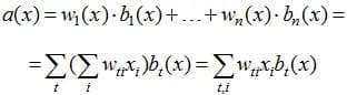
Here weights are sought in the form of linear regressions over the original features. It can be seen that the task of constructing such an ensemble is reduced to setting up linear regression in the space of features, which are all kinds of products of the original features and the answers of the basic algorithms. This method was used by the Top2 Netflix Prize competition team.
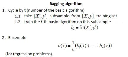
Bagging (bootstrap aggregating)
The idea behind bagging (bootstrap aggregating) is simple: each basic algorithm is trained on a random subset of the training sample. In this case, even using the same algorithm model, we get different basic algorithms. There are the following implementations of the described idea.
The probability of being sampled during bootstrap (a subsample of size m from the main sample of the same size "with return") for sufficiently large samples is approximately 0.632, i.e. approximately 36.8% of objects are “overboard”.
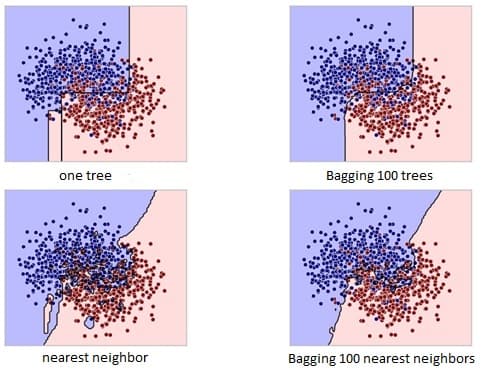
It’s important to understand that subsamples of the training sample are taken in bagging so that the basic algorithms are different. There are models of algorithms that are stable learners with respect to taking subsamples (kNN for k> 3, SVM) and they should not be used in bagging. The figure below shows an attempt to use bagging for a stable algorithm - logistic regression (the upper row is the corresponding bootstrap subsamples and the basic algorithms tuned to them, the lower row is the result of bagging 10 such basic algorithms).
It’s clear that instability is associated with high variance, and small bias should be used, as this guarantees unbiased averaging.
Bagging allows you to receive the so-called out-of-bag (OOB) model responses. The idea is very simple: each algorithm is trained on a subsample, and not all objects of their training fall into the subsample, so the answers of the algorithm can be found on other objects. All constructed algorithms are averaged; by analogy, it is possible to average the responses of algorithms for each learning object, in the training samples of which this object was not included:
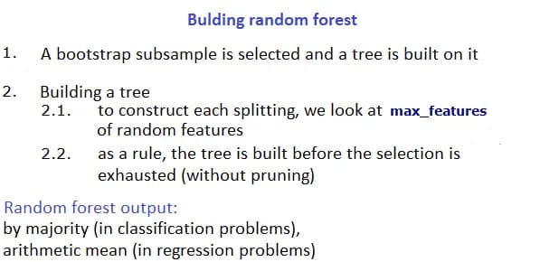
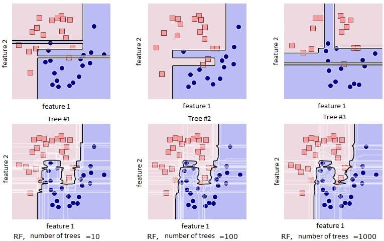
Random Forests
It’s strongly suggested that you check this post first to get more detailed information on random forest.
The algorithm itself combines the ideas of bootstrap and Random Subspaces.
Boosting
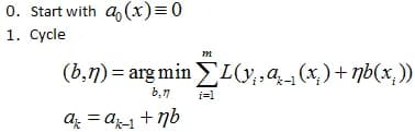
The main idea of boosting is that the basic algorithms are not built independently, we build each next one so that it corrects the mistakes of the previous ones and improves the quality of the entire machine learning ensemble. The first successful boosting option, AdaBoost (Adaptive Boosting), is practically not used these days since it was replaced by a gradient analog. The figure below shows how the weights of objects change when constructing the next basic algorithm in AdaBoost: objects that are classified incorrectly by the first two algorithms have a lot of weight when constructing the third. The basic principle of boosting implementation is Forward Stagewise Additive Modeling (FSAM). For example, let the regression problem be solved with the error function L(y,a). Suppose we have already built an algorithm a(x), now we construct b(x) in such a way that:
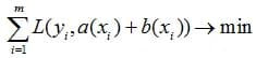
If this idea is applied recursively, we get the following algorithm:
Interesting fact: the peculiarity of terminology when talking about boosting is as follows: basic algorithms are called weak learners, and ensemble is called strong learner. It came from this learning theory.
ECOC ensembles
ECOC stands for Error-Correcting Output Codes and is also used in machine learning. The main idea is to make a special encoding in a problem with l classes using the Error-Correcting Output Code, for example, with *l *= 4:
0 – 000111 1 – 011100 2 – 101010 3 – 110001
Further in this example, we train 6 binary classifiers, according to the number of columns in the binary encoding matrix, each solves the problem with the encoding corresponding to its column. For example, the first one tries to separate objects of classes 0 and 1 from objects of classes 2 and 3.
Suppose we need to classify an object, we run 6 constructed classifiers, write their answers in the form of a binary vector, for example, (1,0,1,0,0,0), look at the Hamming distance to which row of the encoding matrix it is closer. In this case, it’s closer to the line corresponding to class 2. If our code corrects one error, then if one of the classifiers is mistaken, we still return the correct answer.
Homogeneous ensembles
When staking, we built machine learning algorithms that received responses from other algorithms as features, that is, this is a superposition of algorithms. For simplicity, as the basic algorithms and meta-algorithm, you can take the sigmoid from a linear combination of arguments (as in logistic regression). Then you can recursively apply ensemble (i.e. make stacking from stacking), then we get a classic multilayer neural network. But unlike stacking, a neural network, as a rule, is trained not layer by layer, but all at once: the parameters of all neurons (in our terminology - meta-algorithms) are corrected simultaneously iteratively using an analog of the gradient descent method. This is where we're stepping into deep learning soil, so we're going to stop here due to the natural size constraints of a blog post.