ROC AUC compresses a classifier's ranking performance across every decision threshold into one number. That convenience also makes the metric easy to misuse. A sound calculation starts with true and false positive rates, handles equal scores correctly, and keeps model ranking separate from threshold selection. Here is the full derivation, a worked example, and reproducible Python.
The ROC AUC formula at a glance
For a binary classifier and threshold t, first calculate the true positive rate (TPR) and false positive rate (FPR):
TPR(t) = TP(t) / [TP(t) + FN(t)]
FPR(t) = FP(t) / [FP(t) + TN(t)]
TP, FP, TN, and FN mean true positive, false positive, true negative, and false negative. TPR is also called recall or sensitivity. FPR equals 1 - specificity.
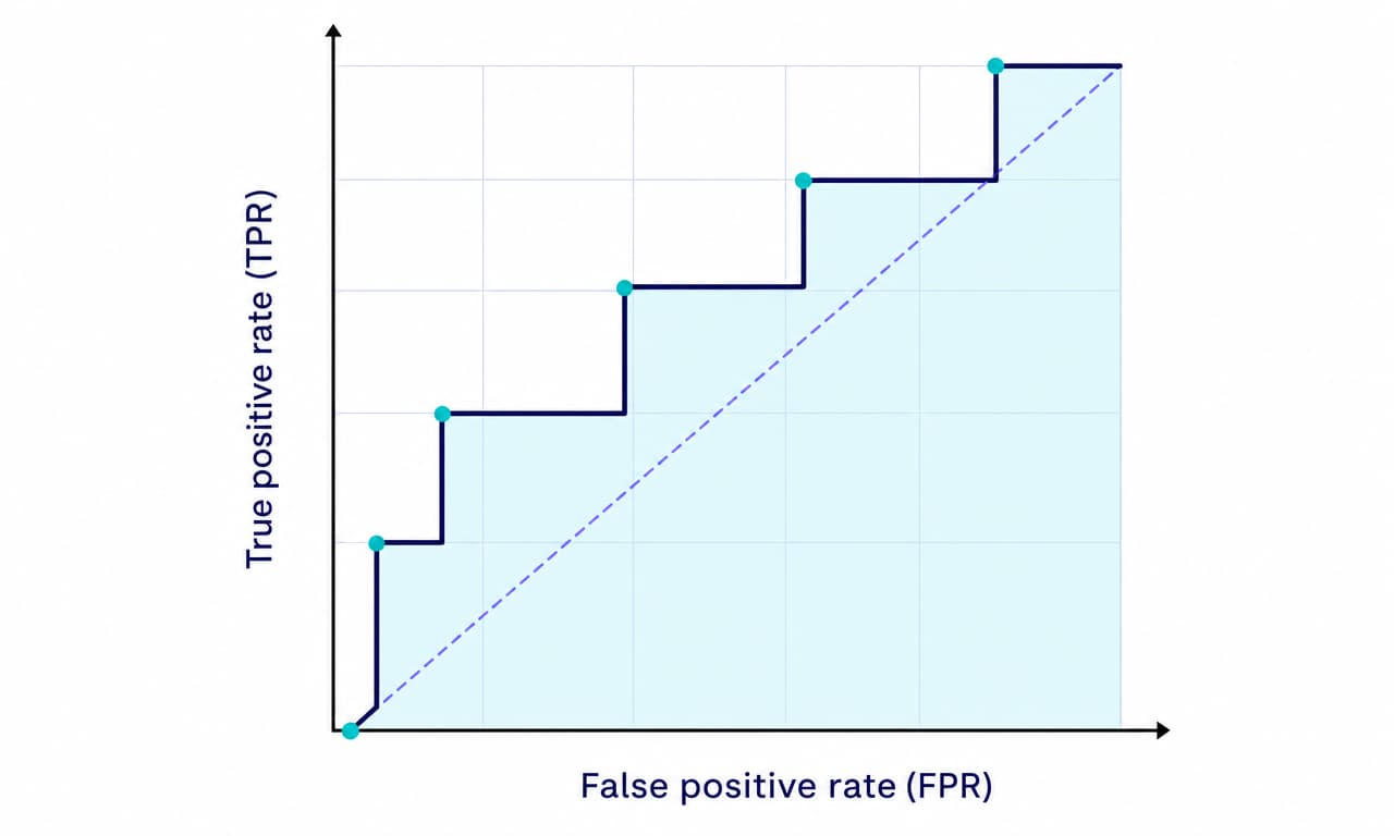
The receiver operating characteristic (ROC) curve contains the points (FPR(t), TPR(t)) produced as t moves through the model's score values. The area under that curve (AUC) is:
AUC = integral from 0 to 1 of TPR(u) du, where u = FPR
For the finite set of points produced by a dataset, sort the ROC points by increasing FPR and apply the trapezoidal rule:
AUC = sum [(FPR_i - FPR_(i-1)) x (TPR_i + TPR_(i-1)) / 2]
An equivalent pairwise formula is often easier to interpret. Let P be the number of positive examples, N the number of negative examples, and s the model score. Then:
AUC = [sum over positive-negative pairs of I(s_pos > s_neg) + 0.5 x I(s_pos = s_neg)] / (P x N)
Here, I(condition) equals 1 when the condition is true and 0 otherwise. Each correctly ordered positive-negative pair earns 1, an equal-score pair earns 0.5, and a reversed pair earns 0. This is why AUC can be read as the probability that a random positive receives a higher score than a random negative, with half credit for ties. Google's ROC and AUC guide gives the same ranking interpretation. The treatment of ties is important for discrete scores and is analyzed directly in a peer-reviewed study of binary predictors.
You can also calculate AUC from ranks. Rank all scores from lowest to highest and assign average ranks to ties. If R_pos is the sum of the positive examples' ranks, then:
AUC = [R_pos - P(P + 1) / 2] / (P x N)
The integral, trapezoidal, pairwise, and rank-sum formulas calculate the same empirical ROC AUC when ties use the standard half-credit convention.
How prediction scores become a ROC curve
A binary model usually emits a continuous score, such as a probability or decision function value. For each threshold, classify scores greater than or equal to the threshold as positive. Lowering the threshold changes the confusion matrix and produces another ROC point.
The process is mechanical:
- Start above the highest score. Nothing is predicted positive, so the curve starts at
(0, 0). - Lower the threshold through the distinct scores in descending order.
- When a positive example enters the predicted-positive set, TPR rises by
1/P. - When a negative example enters, FPR rises by
1/N. - Include every example with the same score at once. A tied group containing both classes creates a diagonal segment.
- Finish below the lowest score. Every example is predicted positive, so the curve ends at
(1, 1).
A vertical move improves recall without adding false positives. A horizontal move adds false positives without finding another positive. Curves that rise toward the upper-left corner therefore enclose more area.
Worked ROC AUC calculation by hand
Consider seven examples with three positives and four negatives:
| ID | Model score | Actual class |
|---|---|---|
| 1 | 0.50 | 0 |
| 2 | 0.10 | 0 |
| 3 | 0.20 | 0 |
| 4 | 0.60 | 1 |
| 5 | 0.20 | 1 |
| 6 | 0.30 | 1 |
| 7 | 0.00 | 0 |
Sort by score and lower the threshold. The two examples scored 0.20 enter together because one is positive and one is negative.
| Threshold | Newly included classes | FPR | TPR |
|---|---|---|---|
infinity | none | 0 | 0 |
| 0.60 | 1 | 0 | 1/3 |
| 0.50 | 0 | 1/4 | 1/3 |
| 0.30 | 1 | 1/4 | 2/3 |
| 0.20 | 0, 1 | 1/2 | 1 |
| 0.10 | 0 | 3/4 | 1 |
| 0.00 | 0 | 1 | 1 |
Apply the trapezoidal formula to consecutive points. Vertical segments have zero width, so they add no area:
AUC = (1/4)(1/3) + (1/4)[(2/3 + 1) / 2] + (1/4)(1) + (1/4)(1)
AUC = 1/12 + 5/24 + 1/4 + 1/4 = 19/24 = 0.7917
The pairwise calculation reaches the same result with less geometry. There are 3 x 4 = 12 positive-negative pairs:
- The positive scored
0.60beats all four negatives: 4 wins. - The positive scored
0.30beats three negatives: 3 wins. - The positive scored
0.20beats two negatives and ties one: 2.5 wins.
That gives 9.5 / 12 = 0.7917. The half point from the tied pair is the detail many hand calculations miss.
Hard class labels are a special case
ROC AUC is most informative when it receives the original scores. A set of hard 0 and 1 predictions has only one nontrivial operating point. Under the standard linear interpolation, its ROC curve connects (0, 0), (FPR, TPR), and (1, 1), so the trapezoidal area reduces to:
AUC_hard = (1 + TPR - FPR) / 2
Since specificity equals 1 - FPR:
AUC_hard = (sensitivity + specificity) / 2
This is balanced accuracy for binary predictions. In the worked example, a threshold of 0.25 gives TPR = 2/3 and FPR = 1/4, so hard-label AUC is 17/24 = 0.7083. Converting the scores to classes discarded useful ordering information and reduced the AUC from 0.7917.
A continuous ROC AUC example
The same formulas work when class scores follow continuous distributions. Suppose negative scores on [0, 1] have density f_0(a) = 2 - 2a, while positive scores have density f_1(a) = 2a.
At threshold t:
TPR(t) = integral from t to 1 of 2a da = 1 - t^2
FPR(t) = integral from t to 1 of (2 - 2a) da = (1 - t)^2
Let x = FPR. Then t = 1 - sqrt(x), which gives the ROC curve TPR(x) = 2sqrt(x) - x. Its area is:
AUC = integral from 0 to 1 of [2sqrt(x) - x] dx = 5/6 = 0.8333
The pairwise view gives the same value. A random positive score exceeds a random negative score with probability 5/6. This equality between geometric area and pairwise ranking probability is the central idea behind ROC AUC.
Calculate ROC AUC in Python
Use roc_auc_score for the scalar metric and roc_curve for the points. Pass scores or positive-class probabilities, rather than predictions returned after thresholding. The current scikit-learn ROC AUC API accepts either probability estimates or non-thresholded decision values for binary classification.
from sklearn.metrics import roc_auc_score, roc_curve

y_true = [0, 0, 0, 1, 1, 1, 0]
y_score = [0.50, 0.10, 0.20, 0.60, 0.20, 0.30, 0.00]

score = roc_auc_score(y_true, y_score)
fpr, tpr, thresholds = roc_curve(
    y_true,
    y_score,
    drop_intermediate=False,
)

print(f"ROC AUC: {score:.4f}")
for threshold, x, y in zip(thresholds, fpr, tpr):
    print(f"threshold={threshold:>4}, FPR={x:.2f}, TPR={y:.2f}")
The result is:
ROC AUC: 0.7917
threshold= inf, FPR=0.00, TPR=0.00
threshold= 0.6, FPR=0.00, TPR=0.33
threshold= 0.5, FPR=0.25, TPR=0.33
threshold= 0.3, FPR=0.25, TPR=0.67
threshold= 0.2, FPR=0.50, TPR=1.00
threshold= 0.1, FPR=0.75, TPR=1.00
threshold= 0.0, FPR=1.00, TPR=1.00
The first threshold is infinity, representing the point where every prediction is negative. drop_intermediate=False keeps collinear points so the output mirrors the hand calculation. Leaving it at the default can remove redundant plotting points without changing the curve's shape or AUC, as the roc_curve documentation explains.
Calculate the metric on held-out data or out-of-fold predictions. Training-set AUC includes memorization and usually gives an optimistic estimate of generalization.
ROC AUC is undefined when the evaluation data contains only one class. Both the rate denominators and the set of positive-negative pairs require at least one positive and one negative.
For multiclass classification, choose the reduction explicitly and pass one score per class:
macro_auc = roc_auc_score(
    y_true,
    y_proba,
    multi_class="ovr",
    average="macro",
)
One-vs-rest (ovr) compares each class with all other classes. One-vs-one (ovo) averages pairwise class comparisons. Macro averaging gives each calculated AUC equal weight, while weighted averaging uses observed class support.
How to interpret a ROC AUC score
ROC AUC measures discrimination, meaning the quality of the model's ordering. It does not measure accuracy at a chosen threshold or the reliability of predicted probabilities.
| ROC AUC | Exact interpretation |
|---|---|
| 1.0 | Every positive receives a higher score than every negative. |
| 0.5 | A random positive is ranked above a random negative half the time. |
| Below 0.5 | The score direction or positive-class coding may be reversed, or the model ranks worse than chance on this sample. |
An AUC of 0.95 means that a random positive receives a higher score than a random negative about 95% of the time, with ties receiving half credit. It does not mean 95% accuracy, 95% precision, or a 95% probability that any one prediction is correct.
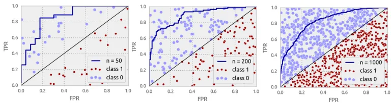
There is no universal cutoff for a "good" AUC. A useful judgment compares the model with a relevant baseline, reports uncertainty, and checks the part of the ROC curve that the application can actually use. An AUC estimated from a small number of either class can vary sharply across samples even when the total dataset looks large.
Choose the operating threshold separately
AUC averages performance across thresholds. Production systems eventually need one threshold, or a small set of policy-specific thresholds.
Choose that operating point on validation data using the actual decision constraints:
- If false positives and false negatives have estimated costs, minimize
cost(t) = c_FP x FP(t) + c_FN x FN(t). - If the system requires at least a given recall, find thresholds that satisfy it and choose the one with the lowest acceptable FPR.
- If sensitivity and specificity receive equal weight, maximizing Youden's
J = TPR - FPRgives the point farthest above the chance diagonal. - Lock the rule before final test evaluation, then monitor it as class prevalence and score distributions change.
Two models can have similar full AUC values and behave very differently in the low-FPR region. Scikit-learn's roc_auc_score supports standardized partial AUC through max_fpr when only that range matters.
When another metric answers the real question better
ROC AUC gives positives and negatives equal weight through pairwise comparisons. That property is useful for ranking, yet it can hide an operationally poor result when positives are rare. A model may achieve a high AUC while generating too many false alerts for the available review capacity. Research comparing the curves found that precision-recall is more informative for many strongly imbalanced classification settings.
| Decision question | Metric or analysis to add |
|---|---|
| How well does the model rank either class across thresholds? | ROC curve and ROC AUC |
| How useful are positive alerts when positives are rare? | Precision-recall curve and average precision |
| Are predicted probabilities numerically trustworthy? | Calibration curve, Brier score, or log loss |
| How does one deployed threshold perform? | Confusion matrix, precision, recall, specificity, and decision cost |
| Do only the first results in a ranked list matter? | Precision at k, recall at k, or another top-weighted ranking metric |
Scikit-learn calculates average precision as a recall-weighted mean of precision across thresholds. It is different from trapezoidal PR area, so name the exact calculation when reporting "PR AUC."
AUC also ignores the numerical spacing between scores. Any strictly increasing transformation preserves their order and therefore preserves ROC AUC. A model can keep the same AUC while its probability estimates become much worse. Use a calibration analysis when the scores drive forecasts or expected-value decisions, and use log loss when you need a proper score for probability quality.
Use ROC AUC as a ranking diagnostic. Pair it with the threshold, cost, calibration, and class-imbalance metrics that describe the decision the model will make.