A graph neural network learns from entities and the relationships between them. That makes GNNs useful for molecules, transaction networks, recommendations, and other problems where connections carry signal. The harder question is whether a graph adds enough information to justify the extra modeling and infrastructure. Here is a practical guide to message passing, GNN architectures, task design, evaluation, and the cases where a simpler model is the better choice.
What is a graph neural network?
A graph neural network, or GNN, is a neural network designed for data represented as a graph. A graph contains entities called nodes and relationships called edges. Both can carry features.
The short answer is that a GNN learns a representation, also called an embedding, for each node by combining that node's features with information from its neighbors. Those embeddings can support predictions about nodes, edges, or an entire graph.
This makes a GNN different from a diagram of a neural network or the computational graph used by an automatic differentiation library. The graph is part of the model's input. Its topology says which entities may exchange information.
| Graph component | What it represents | Transaction-network example |
|---|---|---|
| Node | An entity | Account, card, device, or merchant |
| Edge | A relationship or event | Transfer, login, purchase, or shared device |
| Node feature | Information about an entity | Account age, country, or prior activity |
| Edge feature | Information about a relationship | Amount, timestamp, direction, or event type |
| Global feature | Context for the whole graph | Market, time window, or network-wide condition |
Graphs can be directed or undirected, homogeneous or heterogeneous, static or dynamic. They may have no geometric coordinates at all. Their defining property is relational structure, not a particular visual layout.
How does a graph neural network work?
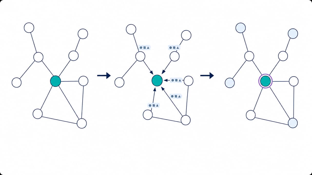
Most modern GNNs use message passing. One layer performs three operations for every node:
- Create messages. Each neighbor contributes information based on its current embedding and, when available, the connecting edge's features.
- Aggregate messages. The model combines the incoming messages with an order-independent operation such as sum, mean, maximum, or learned attention.
- Update the node. A learned function combines the aggregated message with the node's existing embedding.
In compact form:
message(v) = AGGREGATE(M(h_v, h_u, e_uv) for u in neighbors(v))
new_h_v    = UPDATE(h_v, message(v))
Here, h_v is the current embedding of node v, h_u is a neighbor's embedding, and e_uv contains optional edge features. M, AGGREGATE, and UPDATE vary by architecture. The aggregate operation must ignore the order in which neighbor messages arrive. If node IDs are renumbered, node-level outputs should be renumbered in the same way. The PyTorch Geometric message-passing model uses this same structure.
One layer gives a node information from its immediate neighbors. Two layers give it information that has traveled from neighbors of neighbors. In a basic message-passing GNN, k layers therefore create a k-hop receptive field.
A worked message-passing example
Suppose an account sends money to two new recipients. A row-based model can inspect the account's amount, age, and transaction count. A GNN can also learn from the recipients' features and the transfer edges.
After one layer, the account's embedding can reflect whether its direct recipients are new, high-risk, or unusually connected. After two layers, it can reflect patterns around those recipients, such as several accounts converging on the same device. Direction, amount, and time still need to be represented explicitly if they matter. A plain undirected edge would discard them.
The network does not follow a hand-written rule such as “three shared devices means fraud.” Training adjusts the message and update functions so that the resulting embeddings help predict the labeled target.
After message passing, the model uses the embeddings in one of three ways:
- A node head maps each node embedding to a node prediction.
- An edge decoder combines two node embeddings, and sometimes edge features, to score a relationship.
- A readout function pools node embeddings into one graph embedding for a graph-level prediction.
Choose the prediction target before the architecture
“Use a GNN” is incomplete until the unit of prediction is clear. The same data can support different tasks, losses, and evaluation splits.
| Task | Output | Examples |
|---|---|---|
| Node-level | One prediction per node | Classify an account, predict a paper's topic, estimate a mesh point's state |
| Edge-level | One prediction per node pair or edge | Recommend an item, predict a missing link, classify a transaction |
| Graph-level | One prediction per graph | Predict a molecule's property or classify a program's syntax graph |
Graph generation is a related fourth family. It learns to create or edit graph structure, often under constraints. That is different from graph-level prediction, which maps an existing graph to a label or value.
Target choice affects leakage. If the business decision is whether to block a new transfer, an edge-level model evaluated on future transfers is more faithful than a node classifier evaluated on a random sample of historical accounts.
Main GNN architectures and their tradeoffs
Most named GNN architectures change how messages are formed, sampled, weighted, or pooled. Start with the simplest architecture that matches the graph and deployment pattern.
| Architecture | Core idea | Good starting fit | Main tradeoff |
|---|---|---|---|
| Graph convolutional network (GCN) | Degree-normalized neighbor aggregation | Homogeneous graphs and a strong node-classification baseline | Fixed weighting can blur distinct neighbors; full-neighborhood training becomes expensive on large graphs |
| GraphSAGE | Samples neighbors and learns an aggregation function | Large or evolving graphs where the model must embed unseen nodes | Sampling saves work but introduces another source of variance and information loss |
| Graph attention network (GAT) | Learns a weight for each neighbor's message | Neighborhoods where some connections should matter more than others | Attention adds per-edge computation and memory use |
| Graph isomorphism network (GIN) | Uses sum aggregation and a multilayer perceptron to retain structural distinctions | Graph classification and structure-sensitive tasks | Expressiveness does not remove scaling or long-range bottlenecks |
| Relation-aware GNN | Uses separate parameters or transformations for edge types | Knowledge graphs and heterogeneous networks | Parameter count and sampling complexity grow with relation types |
The original GCN paper describes a localized graph convolution whose work scales linearly with the number of edges. GraphSAGE introduced an inductive approach that learns to generate embeddings for unseen nodes by sampling and aggregating neighborhoods. GAT and GIN then changed the aggregation step through learned attention and a more discriminative sum-and-MLP design, respectively.
Architecture names can distract from larger choices. Edge direction, timestamps, relation types, negative sampling, and the train-test split often matter more than replacing one message-passing layer with another.
When a GNN is the right model
A GNN is worth testing when all of these conditions are plausible:
- Relationships carry predictive signal. The target depends on who is connected to whom, not only on each entity's independent attributes.
- The graph has defensible semantics. An edge corresponds to a real relationship, interaction, or proximity rule that can be applied consistently at inference time.
- The topology is irregular. The problem does not fit a simpler grid, sequence, hierarchy, or fixed-size table.
- The required neighborhood is affordable. Relevant evidence can be reached without expanding an unmanageable number of neighbors.
- Evaluation can match deployment. You can hold out future edges, unseen nodes, new graphs, or other cases the model will actually face.
The fastest way to test the first condition is a baseline. Add simple graph features such as degree, counts by neighbor type, recent two-hop counts, PageRank, or connected-component size to a conventional model. Compare that with entity features alone and with a basic GCN. If a random forest baseline matches the GNN, the simpler system is usually easier to train, explain, and serve.
When another model is a better fit
| Data or goal | Start with | Why |
|---|---|---|
| Regular images or spatial grids | Convolutional neural network | The neighborhood and relative positions are fixed |
| Ordered text, audio, or event sequences | Transformer, recurrent model, or temporal convolution | Order and distance already provide structure |
| Independent rows with strong features | Gradient-boosted trees or multilayer perceptron | Graph construction may add cost without signal |
| Exact shortest path, connectivity, or matching | A graph algorithm | The objective already has an exact or well-understood solver |
| Small sets with dense pairwise interactions | Transformer or set model | Learned all-to-all interaction may be simpler than choosing edges |
| Sparse, irregular relational data | GNN | Supplied adjacency constrains information exchange to meaningful connections |
A GNN is not automatically better than a CNN or Transformer. It carries a different inductive bias. A CNN assumes a regular local grid. A standard Transformer learns interactions across a dense token set. A message-passing GNN follows the sparse neighborhood supplied by the graph.
Where graph neural networks are used today
GNNs are still used where relationships are native to the problem. The useful pattern across applications is consistent: the relation is part of the phenomenon being modeled.
Molecular and materials prediction
Atoms become nodes, bonds become edges, and chemical attributes become features. The target may be a molecular property, a bond, or an atomic state. The message-passing neural network paper unified several molecular models around message and readout functions and evaluated them on quantum-chemistry prediction.
Recommendation and retrieval
A recommendation graph often connects users, items, queries, or collections through interactions. Link prediction can rank candidate user-item edges. GraphSAGE demonstrated inductive classification on evolving information graphs, while the later PinSage work applied graph convolutions and importance sampling to a web-scale recommendation setting.
Relational risk and anomaly detection
Accounts, devices, addresses, and merchants form a heterogeneous network. Typed, directed, and time-stamped edges can reveal structures that isolated transaction rows miss. The graph must be built with data available at decision time, or neighborhood features will leak future activity.
Physical systems and forecasting
Mesh points, particles, or geographic cells can be nodes, with edges describing local interaction or proximity. The result can be a node-level forecast over time. GraphCast, for example, used a GNN-based architecture for medium-range global weather forecasting in a peer-reviewed study.
Knowledge graphs
Entities become nodes and typed facts become directed edges. Models can score missing relations or produce entity embeddings for downstream retrieval. A knowledge graph is the data structure. A GNN is one possible model over that structure.
A practical GNN development workflow
1. Write the prediction contract
Define the prediction unit, target, prediction time, allowed input window, and latency budget. State whether inference covers known nodes in a fixed graph, unseen nodes joining an existing graph, or entirely new graphs. These correspond to different transductive and inductive settings.
2. Define the graph before choosing the model
List each node type and edge type. Decide whether edges are directed, weighted, repeated, or time-stamped. Record how you will handle isolated nodes, missing features, duplicate entities, and deleted relationships.
Treat graph construction as a learned-system dependency. A model trained on identity resolution that is unavailable online has no valid serving path.
3. Split data the way production changes
Random splits can place nearly identical neighborhoods, reciprocal edges, or future information on both sides of the evaluation. Use temporal splits for future events, entity-disjoint splits for cold starts, and graph-disjoint splits when the model must generalize to new graphs.
The Open Graph Benchmark was created partly to standardize realistic, application-specific splits and metrics across node, link, and graph tasks. That principle matters on private datasets too.
4. Establish baselines
Train at least three:
- A feature-only model with no graph information.
- A conventional model with hand-built graph statistics.
- A shallow GNN such as a two-layer GCN or GraphSAGE model.
Add complexity only when a baseline exposes a specific gap. Track ablations for node features, edge features, and topology so you know where the gain comes from.
5. Implement the smallest end-to-end model
In PyTorch Geometric, x holds node features and edge_index stores graph connectivity in sparse coordinate form. A two-layer node classifier can be this small:
import torch
from torch.nn import functional as F
from torch_geometric.nn import GCNConv

class NodeGCN(torch.nn.Module):
    def __init__(self, in_channels, hidden_channels, out_channels):
        super().__init__()
        self.conv1 = GCNConv(in_channels, hidden_channels)
        self.conv2 = GCNConv(hidden_channels, out_channels)

    def forward(self, x, edge_index):
        x = self.conv1(x, edge_index).relu()
        x = F.dropout(x, p=0.5, training=self.training)
        return self.conv2(x, edge_index)
The model returns one logit vector per node. Training still needs labels, a loss, and masks that respect the chosen split. The PyTorch Geometric introduction documents the data object, batching model, and basic training flow.
6. Evaluate the system around the score
Measure the metric tied to the decision, then add operational checks:
- Performance by node degree, relation type, time period, and seen versus unseen entities
- Calibration when scores trigger risk or ranking thresholds
- Training memory, neighbor-sampling cost, inference latency, and embedding freshness
- Sensitivity to missing, delayed, or noisy edges
- Gains over feature-only and graph-feature baselines
- Learning curves to distinguish data limits from optimization problems
An aggregate accuracy or area-under-curve score can hide a model that fails on isolated nodes or the newest part of the graph.
Common GNN limitations
Graph quality becomes model quality
Wrong entity merges, missing edges, stale links, and arbitrary proximity thresholds change the model's input structure. More message passing can amplify those errors. Version the graph-building logic and monitor graph statistics alongside model metrics.
Neighborhoods grow quickly
High-degree nodes and multiple hops can expand the computation far beyond the seed batch. Sampling caps work, but it can omit rare, important neighbors and makes training stochastic. Large graphs often need dedicated graph storage, sampling, and embedding-refresh paths.
Deep message passing can erase distinctions
Repeated neighbor averaging can make nearby node embeddings increasingly similar. This is called over-smoothing. A Laplacian smoothing analysis identified this as a limit of deep graph convolution. Fewer propagation layers, residual connections, and separating feature transformation from propagation are common responses.
Long-range evidence can be compressed away
A fixed-size embedding may need to carry information from an exponentially growing set of distant nodes. This over-squashing bottleneck makes long-range dependencies difficult even before over-smoothing appears. The original bottleneck study showed that popular message-passing models can fail to fit tasks that depend on distant signals.
Neighbor similarity is not universal
Basic convolution works well when connected nodes tend to have compatible labels or features. Some graphs connect opposites, such as buyers and sellers or attackers and targets. Typed relations, direction-aware messages, positional or structural features, and heterophily-aware models may fit better than a vanilla GCN.
Evaluation leakage is unusually easy
The graph ties examples together. A future edge can expose the outcome of an earlier node, and a random link split can leave the reverse edge or same entities in training. Build every neighborhood from information available at the simulated prediction time.
Do large language models use graph neural networks?
Most large language models use Transformer architectures. A Transformer layer can be interpreted as message passing over a fully connected token graph, but a standard LLM does not consume an arbitrary graph's adjacency and edge types the way a GNN does. Hybrid systems can combine an LLM with a knowledge graph or GNN when explicit relations add useful context.
Start with the graph, then earn the neural network
The decisive work in a GNN project happens before the first layer: define meaningful nodes and edges, prevent time leakage, choose the true prediction unit, and establish a simple baseline. Message passing is valuable when neighboring evidence changes the answer.
Sketch the graph schema and production split first. Then make a shallow GNN beat feature-only and graph-statistic baselines before you invest in deeper architecture or graph infrastructure.