Surprisingly, it is extremely difficult to find a good overview of all the methods of model calibration - a process as a result of which the “black boxes” not only qualitatively solve the classification problem, but also correctly assess their confidence in the answer given.
This calibration machine learning review is not an entry-level one - it is necessary to understand how classification algorithms work and are used, although the author has greatly simplified the presentation, for example, by dispensing with conditional probabilities in the definitions (due to which the rigor of the presentation has suffered a little).
Confidence Calibration Problem in Machine Learning
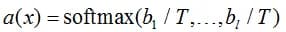
One of the interesting and not fully resolved theoretical and practical problems in machine learning is Confidence Calibration problem. Suppose we are solving a classification problem with l classes, our algorithm produces some estimates of the belonging of objects to classes - Confidences, and then assigns the object to the class with the highest score (i.e., it gives an answer of which we are most confident):
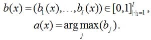
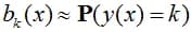
A question naturally arises here: what is the probability that the answer is correct? We would like to be able to evaluate it at the stage of forming a response. The most obvious and "convenient" option - this probability is equal to the maximum estimate (confidence):
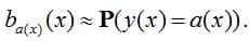
If the equality holds with sufficient accuracy, then the classifier is said to be (well-) calibrated. There may be a more stringent calibration condition - that all estimates correspond to probabilities for each k:
For example, if the classifier for the classes "cat", "dog", "gopher" received confidence (0.8, 0.2, 0.0), then with a probability of 0.8 the correct class is "cat", and with a probability of 0.2 - a "dog" and it’s certain that the object cannot belong to the class "gopher".
Importance of Confidence Score Machine Learning
The confidence score falls between 0 and 1 with the higher number the more likely the result of the model matching the user’s request. So, the confidence score in machine learning is important for various reasons including:
- Correct understanding of how much the results of the algorithm can be trusted. This is important when interpreting models, as well as for making decisions about the implementation of artificial intelligence (AI) systems and analyzing their work.
- For a more accurate solution of AI problems in general, because certainties are often used by other algorithms, for example, in language models, when generating texts, the probabilities of the appearance of individual tokens are used (for example, when using beam search).
- For setting on the so-called scoring loss-funcions, one of which is logistic (in this post I discussed the topic of calibration).
Model Calibration Machine Learning
Let’s describe the way to evaluate the calibration of an algorithm in practice. It is necessary to compare confidence and accuracy on the test sample: bk(x) vs P(y(x)=a(x)). It is clear that if for a large group of objects the algorithm gave an estimate of 0.8 for the class "dog", then in the case of "good calibration" there will be about 80% of objects of this class among them. In practice, the problem is that it is unlikely that for a large group of objects the answer will be exactly 0.8 (and not 0.81, 0.8032, etc.). Therefore, the comparison is made by dividing objects into groups - or bins, in other words:
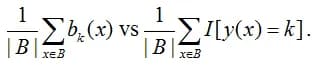
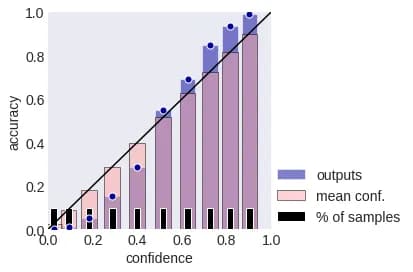
Here, the average of the estimates that fall into a particular bin is compared with the average of the event indicators that the object belongs to the kth class, i.e. with accuracy if we consider k = a (x). These values are usually depicted on the so-called Reliability Plot:
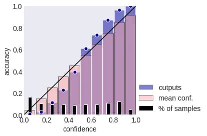
In machine learning calibration, bins are often chosen with borders [0, 0.1], [0.1, 0.2], etc. In the figure above, the pink bars are the obtained mean confidences, and the blue bars are the accuracies in the corresponding bins. The fraction of objects in the sample that fell into the corresponding bin is shown in black. It is clear that the larger the share, the more reliable the estimates of confidence and accuracy. If the blue bar is higher than the pink one, they are talking about under-confidence, if below - about excessive confidence or over-confidenсe.
Calibration is numerically evaluated using Expected Calibration Error (ECE):
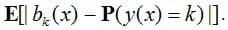
More precisely, ECE is usually estimated by averaging over bins, or more often weighted by "bin frequency":
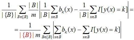
(note that all formulas are given for a fixed class k). Sometimes the multiplier highlighted in red is not used. More often the bins are chosen "of equal width", but the more preferable option - equal capacity, then the quality metric is called daECE (Adaptive ECE). The figure below shows a calibration diagram for equal power bins.
It is clear that the described metrics correspond to the weighted average of the differences between the blue and pink columns. The maximum is sometimes used instead of the average, the corresponding metric is called Maximum Calibration Error (MCE). Also, the calibration is estimated by standard error functions: negative log-likelihood (NLL) and Brier score (as MSE is often called in the classification):
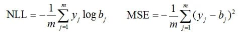
(yj here are the binary values of the object classification, bj is the assessment of belonging to the j-th class).
Modern neural networks are uncalibrated!
They are more likely to suffer from being over-confident. Firstly, this happens because when training neural networks on calibration set, accuracy is monitored, not paying attention to confidence. The figure below shows graphs of different metrics when training neural networks. Secondly, modern networks are very complex, which leads to overfitting (even if NLL decreases on the training set when the network is trained, on the test set the NLL can increase, (see the figure below).
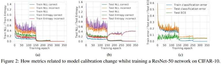
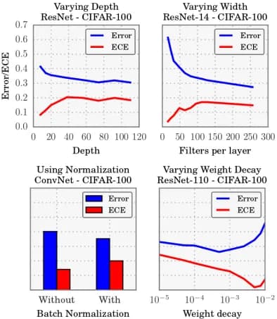
Thirdly, most of the modern techniques used in DL (large depth, normalization by batches, etc.) worsen calibration, as you can see from the figure below.
Model Calibration Methods Machine Learning
Below we will discuss the basic calibration methods. Note that it is usually performed on a calibration set. Most of the methods replace the answer of the algorithm, more precisely, the confidence of the answer: the biased estimate is replaced by a value that is closer to accuracy. The function that performs this substitution is called the deformation function.
Histogram binning
The following optimization problem is solved by {θi} parameters
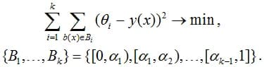
Initially, bins of the same width were used in this method (but equally powerful ones can be also used). After solving the problem, if the assessment of belonging to the class fell into the i-th bin, it is replaced with the corresponding value θi. Cons of this approach:
- the number of bins is set in the very beginning,
- the deformation function has no continuity,
- in the “equal-width version,” some bins contain a small number of points.
This method was proposed in the work of Zadrozny В., Elkan C. «Obtaining calibrated probability estimates from decision trees and naive bayesian classifiers». In ICML, pp. 609–616, 2001.
Method for transforming classifier scores to accurate two-class probability estimates
Here a monotonically non-decreasing deformation function of the algorithm estimates is constructed. In fact, the same optimization problem is solved as in the method 1, but there is an additional condition:
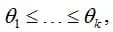
optimization is carried out with respect to the parameters k, {θi}, {αi}. By the way, this problem is solved by the pool adjacent violators algorithm (PAV / PAVA) in linear time O(N).
This method was proposed in the work of Zadrozny, Bianca and Elkan, Charles. Transforming classifier scores into accurate multiclass probability estimates. In KDD, pp. 694–699, 2002.
As before, the deformation function is not continuous. Approaches to smoothing it are suggested here
Platt Calibration
Initially, the method was developed for SVM, the estimates of which lie on the real axis (in fact, these are the distances to the optimal line separating the classes, taken with the required sign); it is believed that the method is not very suitable for other models (although it has many generalizations). Let the algorithm outputs the signed distance to the dividing surface r(x), and we look for a solution as follows:
parameters are determined by the method of maximum likelihood on the calibration set.
(Also take a look at: Platt, John et al. Probabilistic outputs for support vector machines and comparisons to regularized likelihood methods. Advances in large margin classifiers, 10(3): 61–74, 1999)
Matrix and Vector Scaling
It is a set of parametric methods with one idea, which is displayed in the title. The first method, which is Matrix and Vector Scaling, is a generalization of Platt calibration.
here W is a tunable l×l matrix and b is the translation vector.
(Tim Leathart, Eibe Frank, Bernhard Pfahringer, Geoffrey Holmes «On Calibration of Nested Dichotomies»)
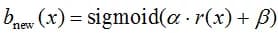
Beta Calibration
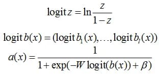
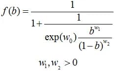
Another method is Beta calibration, in which the deformation in a problem with two disjoint classes is sought in the form as shown below, for which a logistic regression is configured in a space with two features* ln(bi), -ln(1-bi)* and the original target a feature, here bi is an assessment of belonging to class 1 of the i-th object. The rationale for this technique is easy to understand yourself or see in the original work.
The method was further developed in the work of Kull, M. et. al. Beyond temperature scaling: Obtaining well-calibrated multi-class probabilities with Dirichlet calibration. InProceedings of Advances in Neural Information Processing Systems, pp. 12295–12305, 2019.
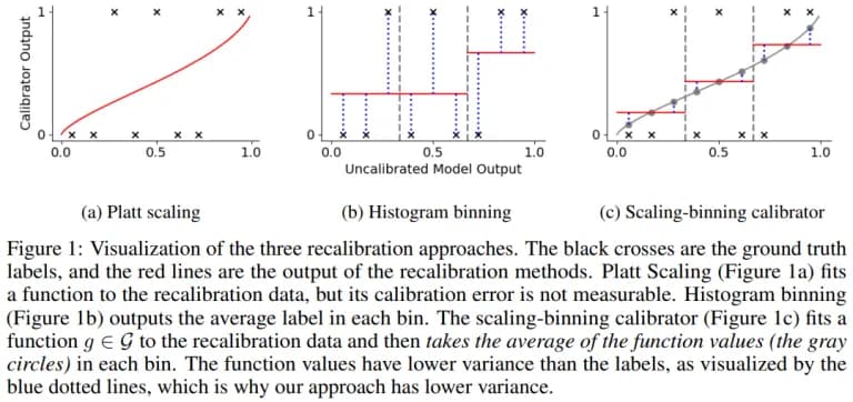
Scaling-binning calibrator
This method combines the binning and parametric methods. First, a parametric deformation curve is built, then binning is performed - already by its values. In the original, one calibration set is used to train the calibration curve in machine learning, the second is used to organize binning, and the third is used for the final calculation of the deformation values.
The fig. below shows the idea of the method by Kumar, Ananya and Liang, Percy S and Ma, Tengyu «Verified Uncertainty Calibration» // Advances in Neural Information Processing Systems 32, 2019, P. 3792-3803
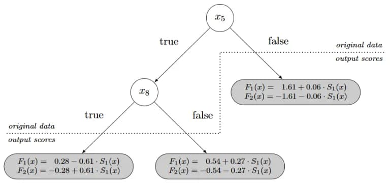
Probability Calibration Trees
As in other machine learning (ML) problems, trees are also used for calibration, the standard algorithm builds a superposition of a tree based on the initial features and logistic regressions (each in its own leaf) over the estimates of the algorithm:
- Build a decision tree (not very deep) based on the initial features.
- In each leaf, train logistic regression on one feature - on the estimates of the calibrated algorithm.
- Prune the tree to minimize the error (the original article used the Brier score).
Again, since there are ensembles everywhere, they are also in the calibrations. One of the popular methods is BBQ (Bayesian Binning into Quantiles), which combines several binnings (equally powerful) with different numbers of bins. The answer is sought in the form of a linear combination of binning estimates with weights; Bayesian averaging is applied. We will not write out the "tricky formulas", but we will redirect the reader to the work of Naeini, M., Cooper, G., Hauskrecht, M.
Ensemble of near isotonic regression (ENIR)
With a slight stretch, we can say that BBQ evolved into ENIR (ensemble of near isotonic regression). This method ensembles “near isotonic regressions” and uses the Bayesian information criterion (BIC). In some review articles, when compared, this method was found to be the best.
Multidimensional generalization of Platt scaling
This method belongs to the class of DL calibration methods, not because it is used exclusively in neural networks, it was just invented and gained popularity precisely for calibrating neural networks. The method is a simple multidimensional generalization of Platt scaling:
Note that the classification result does not depend on the value of the parameter T, which is called "temperature", therefore the accuracy of the calibrated algorithm does not change. As before, the parameter is trained on the calibration set. The main disadvantage of the method is that we simultaneously reduce the confidence in incorrect predictions and in correct ones (take a look at this article).
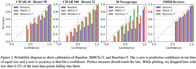
Maximum Mean Calibration Error (MMCE)
This method uses a trick: the MMCE regularizer is introduced, which corresponds to the error in the space deformed with the help of the kernel (earlier, a similar technique was used to compare distributions [Gretton, 2012]). Temperature scaling is also used, in figure below, an illustration of the method from the Aviral Kumar, Sunita Sarawagi and Ujjwal Jain’s article is shown.
Label smoothing
As you might expect, “label smoothing,” as described by Rafael Müller, Simon Kornblith, Geoffrey Hinton, “When Does Label Smoothing Help?” should help combat over-confidence.
If the object belongs to the j-th class, then it corresponds to the classification vector
when setting up a neural network, the cross-entropy between the evaluation vector and the "smoothed classification vector" is minimized
This setting is often combined with temperature scaling.
While battling over-confidence, it is possible to smooth out the answers in the process of training the network, for this it is natural to use entropy, which is maximum when the confidences for all classes are equal and minimum, when we are confident in only one particular class. It is logical to subtract the entropy from the error function with some coefficient and mimic the obtained expression by backward propagation of the gradient. You can learn more on that by following this link
Focal Loss
Focal Loss is an error function for training neural networks proposed by Lin et al. to solve the problem of class imbalance, but it turns out that it might be. used for neural network calibration:
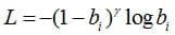
(the error here was written for an object that belongs to the i-th class). It can be shown that it estimates from above the Kullback-Leibler divergence between the target distribution and the network response, from which the response distribution entropy multiplied by the gamma coefficient is subtracted, i.e. the method is similar in nature to the previous two:

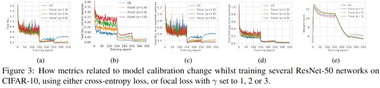
The above methods can be combined, for example, after the optimization of the focal error, in the original work, again, temperature scaling was used. The figure below shows how different metrics changed while minimizing the focal error.
Structured Dropout
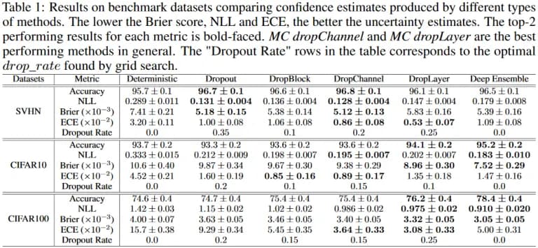
Unlike many other deep learning (DL) tricks, the DropOut helps in the calibration problem, as you can see from the table taken from the article.
We do not provide any comparisons of all the listed methods. There is no research article in which they are all tried on equal terms.
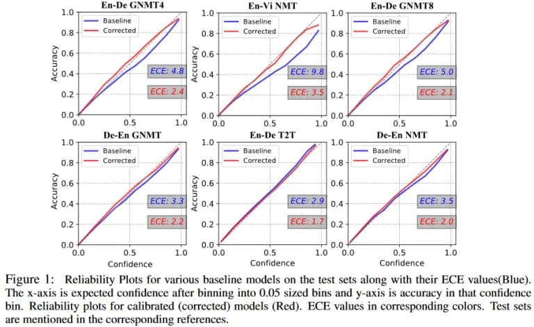
In conclusion, a small review of the research paper by Aviral Kumar and Sunita Sarawagi so that there is no impression that calibration is an exclusively theoretical problem. In the work, we experimented with available (there is an open implementation) and modern models:
- NMT [Bahdanau et al., 2015],
- GNMT [Wu et al., 2016],
- Transformer model [Vaswani et al., 2017].
It used its own "weighted" version of ECE (which we will not describe in detail). The authors concluded that in language models the following is true:
-
the calibration is especially bad for the EOS class (end of sequence marker). This conclusion can be slightly questioned since this class is quite rare (in comparison, for example, with punctuation marks) and it is difficult to assess the true extent of uncalibration. In addition, in different pairs of languages (for translation) it turned out differently: under-calibration or over-calibration.
-
poor calibration is due to the so-called attention uncertainty.
If we use the attention mechanism, then we calculate the attention rates. If some coefficient is much larger than others, then attention is focused (we “look” at a certain token), if all coefficients are approximately equal, then attention is “blurred”. Again, it is logical to formalize such blurring with the help of entropy. It turned out that at its high values and ECE, on average, more, i.e. confidence is rated worse.
The method for solving the calibration problem here is quite original. The temperature scaling method is applied, but the temperature is not constant, but depends on
- attention uncertainty
- the logarithm of the token probability,
- token categories (for example, "EOS"),
- input coverage - the proportion of input tokens with attention above the threshold.
We learn the temperature using the NS (even a few simple NS - they are included in the formula, which we will not give). As a result, it turns out not only to build a calibrated language model (see figure below), but also to improve the quality of translation (BLEU is almost always better).