
Log loss measures how well a classifier's predicted probabilities match observed outcomes. It rewards estimates that assign more probability to the true class and sharply penalizes confident errors. That makes it useful for training and evaluating probabilistic classifiers, where accuracy alone hides too much. Here is the formula, a worked calculation, reliable Python implementations, and the baseline you need to interpret the result.
What is the log loss function?
Log loss is a loss function and evaluation metric for probabilistic classification. For each example, it takes the negative logarithm of the probability that the model assigned to the true class. The dataset score is usually the mean of those per-example losses.
Lower is better. The mathematical range is 0 to infinity. A perfect probability of 1 for every true class produces a log loss of 0. A probability near 0 for the true class produces a large loss. An exact probability of 0 produces infinite loss in the mathematical definition.
Log loss is also called logarithmic loss, logistic loss, cross-entropy loss, or negative log-likelihood in closely related contexts. The names emphasize different views of the same calculation.
| Probability assigned to the true class | Per-example log loss |
|---|---|
| 0.99 | 0.010 |
| 0.90 | 0.105 |
| 0.60 | 0.511 |
| 0.50 | 0.693 |
| 0.10 | 2.303 |
| 0.01 | 4.605 |
The table uses the natural logarithm. Moving from 0.90 to 0.99 saves about 0.095 loss. Moving from 0.10 to 0.01 adds about 2.303. This asymmetry is why a few confident mistakes can dominate the mean.
The binary log loss formula
For one binary example, let:
- y be the observed label, either 0 or 1
- p be the predicted probability that y = 1
The loss is:
L(y, p) = -[y ln(p) + (1 - y) ln(1 - p)]
Because y can only be 0 or 1, one term always disappears:
If y = 1:  L = -ln(p)
If y = 0:  L = -ln(1 - p)
For N examples, average the individual losses:
Log loss = -(1/N) Σᵢ₌₁ᴺ [yᵢ ln(pᵢ) + (1 - yᵢ) ln(1 - pᵢ)]
Most machine learning libraries use the natural logarithm, so scores are measured in nats. Another log base only multiplies every score by a constant. It does not change which model has the lower loss, but you must use the same base when comparing values.
A worked log loss example
Suppose a binary classifier makes four predictions:
| Example | True label y | Predicted P(y=1) | Probability on true class | Loss |
|---|---|---|---|---|
| 1 | 1 | 0.90 | 0.90 | 0.105 |
| 2 | 0 | 0.20 | 0.80 | 0.223 |
| 3 | 1 | 0.60 | 0.60 | 0.511 |
| 4 | 0 | 0.10 | 0.90 | 0.105 |
The mean is:
(0.105 + 0.223 + 0.511 + 0.105) / 4 = 0.236
All four predictions are correct at a 0.5 threshold, so accuracy is 100%. A more hesitant model that predicts 0.60 for both positive examples and 0.40 for both negative examples also gets 100% accuracy. Its log loss is 0.511. Log loss separates models that accuracy treats as identical.
Why log loss works for probabilities
The logarithm gives log loss three useful properties.
It makes confidence matter
At a 0.5 threshold, accuracy sees probabilities of 0.51 and 0.99 as the same positive prediction. Log loss gives them losses of 0.673 and 0.010 when the label is positive. It also distinguishes a cautious error from a confident one. A positive example predicted at 0.49 costs 0.713; the same example predicted at 0.01 costs 4.605.
It rewards honest probability estimates
Log loss is a strictly proper scoring rule. In expectation, the best strategy is to report the probability you actually believe. If an event occurs 70% of the time for a group of examples, predicting 0.70 minimizes expected log loss for that group. The probability calibration guide explains why a proper score reflects both calibration and the model's ability to separate classes.
This matters for forecasts used downstream. A model that says 0.80 should be right about 80% of the time among comparable predictions if those probabilities are well calibrated.
It is negative log-likelihood
For independent binary outcomes, the Bernoulli likelihood of the observed labels is:
Likelihood = Π pᵢ^(yᵢ) (1 - pᵢ)^(1 - yᵢ)
Taking the logarithm turns the product into a sum. Negating and averaging that sum gives binary log loss. Maximizing the likelihood is therefore equivalent to minimizing log loss.
This connection explains its use in logistic regression. If z is the model's raw score and p = sigmoid(z), the derivative of the per-example loss with respect to z simplifies to:
dL/dz = p - y
The gradient moves an overestimated probability down and an underestimated probability up. Its size grows with the probability error.
Is log loss the same as cross-entropy?
For standard classification with one-hot targets, yes. Cross-entropy between a target distribution y and a predicted distribution p is:
H(y, p) = -Σ yₖ ln(pₖ)
A one-hot target has one entry equal to 1. The expression reduces to the negative log probability of the true class, which is the per-example log loss.
The terminology changes with context:
- Binary cross-entropy is the binary formula with p and 1 - p.
- Categorical cross-entropy is the multiclass formula over mutually exclusive classes.
- Negative log-likelihood describes the same objective from the statistical model's likelihood.
- Logistic loss can also mean the equivalent margin form used to train logistic regression.
The reduction matters. A library may return the sum, mean per example, or mean across examples and labels. Check that setting before comparing results from two implementations.
Multiclass log loss
For K mutually exclusive classes, each example has a probability vector whose entries sum to 1. If yᵢ is the index of the true class, multiclass log loss is:
Log loss = -(1/N) Σᵢ₌₁ᴺ ln(pᵢ,ᵧᵢ)
For example, assume the true labels are cat, dog, and fish. The model assigns their true classes probabilities of 0.70, 0.80, and 0.60. The score is:
[-ln(0.70) - ln(0.80) - ln(0.60)] / 3 = 0.364
The other class probabilities still matter because all entries in each row must form one distribution. Increasing one class's probability requires taking probability mass from another class.
Multilabel classification is different. Several labels can be true at once, so each label is usually treated as its own binary outcome. Apply binary cross-entropy across labels, with a reduction that matches the question you want the metric to answer.
How to calculate log loss in Python
NumPy implementation
This implementation makes each numerical step explicit:
import numpy as np

def binary_log_loss(y_true, y_proba):
    y = np.asarray(y_true, dtype=float)
    p = np.asarray(y_proba, dtype=float)

    if y.shape != p.shape:
        raise ValueError("y_true and y_proba must have the same shape")
    if np.any((p < 0) | (p > 1)):
        raise ValueError("probabilities must be between 0 and 1")

    eps = np.finfo(float).eps
    p = np.clip(p, eps, 1 - eps)
    return -np.mean(y * np.log(p) + (1 - y) * np.log1p(-p))

y_true = [1, 0, 1, 0]
y_proba = [0.90, 0.20, 0.60, 0.10]

print(binary_log_loss(y_true, y_proba))  # 0.2361725516
Clipping prevents ln(0) from producing infinity in finite-precision code. It is an implementation safeguard. It does not change the mathematical fact that assigning zero probability to an event that occurs has infinite loss.
scikit-learn implementation
Use sklearn.metrics.log_loss for evaluation:
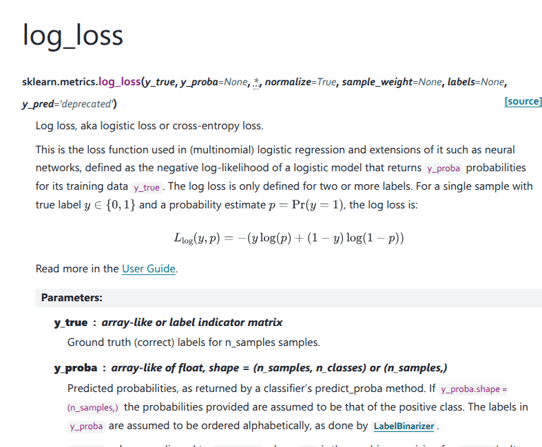
The function accepts one positive-class probability per sample in binary classification, or one probability column per class in multiclass classification.
from sklearn.metrics import log_loss

y_true = [1, 0, 1, 0]
y_proba = [0.90, 0.20, 0.60, 0.10]

score = log_loss(y_true, y_proba)
print(score)  # 0.2361725516
For multiclass predictions, pass one probability column per class:
from sklearn.metrics import log_loss

y_true = ["cat", "dog", "fish"]
y_proba = [
    [0.70, 0.20, 0.10],
    [0.10, 0.80, 0.10],
    [0.20, 0.20, 0.60],
]

score = log_loss(
    y_true,
    y_proba,
    labels=["cat", "dog", "fish"],
)
print(score)  # 0.3635480397
When probabilities come from model.predict_proba(X), keep the columns in model.classes_ order and pass labels=model.classes_. A class-order mismatch can produce a plausible number for the wrong mapping.
Train from logits in PyTorch
During training, compute the loss from raw logits rather than applying a sigmoid or softmax first. BCEWithLogitsLoss combines binary cross-entropy with the sigmoid calculation and uses the log-sum-exp trick for numerical stability.
import torch

logits = torch.tensor([2.20, -1.39, 0.41, -2.20])
targets = torch.tensor([1.0, 0.0, 1.0, 0.0])

loss_fn = torch.nn.BCEWithLogitsLoss()
loss = loss_fn(logits, targets)
print(loss.item())
For one-of-K multiclass targets, use torch.nn.CrossEntropyLoss with raw logits and integer class indices. Applying sigmoid or softmax before these combined losses changes the calculation and can make optimization numerically weaker.
What is a good log loss value?
There is no universal cutoff. Zero is perfect and lower is better, but class prevalence changes the difficulty and the natural baseline.
Compare the model against a constant classifier that always predicts the observed class proportions on the evaluation set. For a binary dataset with positive rate r, that baseline has log loss:
Baseline = -[r ln(r) + (1 - r) ln(1 - r)]
| Positive rate | Constant prediction | Baseline log loss |
|---|---|---|
| 50% | 0.50 | 0.693 |
| 10% | 0.10 | 0.325 |
A score of 0.40 beats the uninformed baseline on the balanced dataset. It loses to the baseline on the dataset with 10% positives. That is why quoting a log loss without the class distribution or baseline says little.
You can express improvement over baseline as a fraction:
D² log loss = 1 - (model log loss / baseline log loss)
A value of 0 matches the constant model, a positive value improves on it, and a negative value is worse. Scikit-learn exposes this calculation as d2_log_loss_score.
For a fair comparison, use the same examples, labels, probability definition, log base, sample weights, and reduction. Compare validation or test loss rather than training loss.
Log loss compared with related metrics
| Metric | What it measures | What it misses |
|---|---|---|
| Log loss | Probability assigned to the observed class | Does not isolate ranking or calibration by itself |
| Accuracy | Fraction of hard labels that are correct at one decision rule | Ignores probability confidence |
| ROC AUC | Ranking of positives above negatives across thresholds | Ignores the probability scale and calibration |
| PR AUC | Precision-recall tradeoff, often informative for rare positives | Ignores whether a score of 0.8 behaves like an 80% probability |
| Brier score | Squared probability error | Penalizes extreme mistakes less sharply than log loss |
Use log loss when the probability itself drives a decision, such as risk scoring, ranking with expected value, forecasting, or choosing among actions with different costs. Pair it with threshold metrics when the deployed system ultimately takes a discrete action.
A lower log loss can come from better class separation, better calibration, or both. Inspect a reliability diagram when you need to diagnose calibration specifically. Post-hoc calibration can improve probabilities when a model ranks examples well but overstates confidence. Experiments on image and document classifiers found temperature scaling effective across many tested neural networks. Fit any calibrator on held-out or cross-validated predictions.
Common log loss mistakes
- Passing hard labels instead of probabilities. Values of exactly 0 and 1 turn each mistake into an extreme penalty. Use predict_proba, calibrated scores, or logits with the framework's combined loss.
- Mapping probability columns to the wrong classes. Preserve the estimator's class order and test it explicitly, especially when string labels are involved.
- Applying sigmoid or softmax twice. Combined training losses expect logits. Evaluation metrics usually expect probabilities.
- Ignoring numerical stability. Clip only when evaluating probabilities. During training, use a loss that operates directly on logits.
- Comparing weighted and unweighted scores. Class weights and sample weights change the quantity being averaged. Report the weighting scheme and keep it fixed across models.
- Reading log loss as a calibration-only metric. A lower score may reflect sharper class separation. Use calibration curves to examine reliability.
- Using the training set for evaluation or calibration. Both practices produce optimistic estimates. Use unseen data and fit calibration as a separate held-out or cross-validated step.
Treat log loss as a score for probability forecasts. Compare it on the same unseen examples, benchmark it against the class-prior baseline, and inspect calibration and decision metrics alongside it. That turns a bare loss value into an evaluation you can act on.