Self-supervised learning creates training targets from structure already present in data. It powers familiar techniques such as masked-token prediction, image-patch reconstruction, and masked speech modeling. The key engineering question is which signal trains each stage, what representation the model learns, and how that representation performs on the downstream task. These examples make those choices concrete across text, vision, speech, and multimodal data.
What is self-supervised learning?
Self-supervised learning (SSL) trains a model with targets or relationships derived from the observed data itself. A hidden word, a missing image patch, the next audio segment, or a second view of the same object can supply the training signal. A person does not have to annotate each pretraining example with a task label.
The usual goal is a useful representation, an embedding or internal feature set that preserves information needed later. The automatically constructed objective is often called a pretext task. A downstream task is the real application used to evaluate or adapt the representation, such as document classification, object detection, or automatic speech recognition.
Modern SSL does not always create a class-style pseudo-label. Reconstruction, alignment, and latent-prediction losses can train an encoder directly.
Worked example: predict a masked word
Start with a sentence from an ordinary text corpus:
The caller moved the appointment to Tuesday.
The data pipeline replaces one token with a mask:
The caller moved the appointment to
[MASK].
The original token, Tuesday, is already available in the source sentence, so it becomes the target automatically. The model reads the surrounding words, predicts a probability distribution over tokens, and updates its parameters when the prediction differs from the original. Repeating this across a large corpus teaches context-sensitive representations.
BERT's pretraining setup is a well-known masked-language example. A downstream classifier can later fine-tune the encoder with labeled intent or topic examples. That distinction matters: label-free pretraining does not mean zero labels, curation, or human supervision throughout the complete pipeline.
Self-supervised learning examples across modalities
The same operational test works across data types: identify the observed input, the automatically available target or relation, and the downstream behavior that will justify the pretraining cost.
| Modality | Observed data | Training signal created from the data | Representative method | Possible downstream use |
|---|---|---|---|---|
| Text | Unlabeled sentences or documents | Hide a token or span and predict it; predict the next token from earlier tokens | BERT masked-token prediction | Classification, retrieval, question answering |
| Vision | Images without class labels | Hide patches and reconstruct them; align two augmented views of one image | Masked Autoencoders and SimCLR | Classification, detection, segmentation |
| Speech/audio | Raw audio without transcripts | Mask latent frames and identify learned acoustic targets; predict clustered units | wav2vec 2.0 and HuBERT | Speech recognition, speaker or acoustic tasks |
| Multimodal | Corresponding observations, such as video and audio | Align synchronized pairs or predict masked units using another modality | AV-HuBERT | Audio-visual speech recognition and robust speech features |
Text: masked, denoising, and next-token objectives
Text supplies order and context without a separate annotation pass. Word2vec used nearby words to learn static word vectors. BERT masks tokens and predicts their originals. T5 corrupts spans and trains an encoder-decoder to reconstruct them. Causal language models predict the next token from the preceding sequence.
These objectives are related, but they are not interchangeable. A masked encoder can use context on both sides of a gap. A causal decoder must predict from the prefix. A language model may also undergo supervised fine-tuning or preference-based post-training after self-supervised pretraining. The training stages should be named separately instead of labeling the entire model pipeline self-supervised.
Vision: reconstruct pixels or match views
A masked autoencoder divides an image into patches, hides a large subset, and reconstructs the missing pixels from the visible patches. The original image provides the target. In contrast, SimCLR creates two augmented views of an image and trains their representations to agree while treating views of other images as negatives.
Both methods can start without class labels. They impose different assumptions. Reconstruction rewards recovery of missing content. View matching rewards invariance to the chosen crops, colors, and other augmentations. The better objective depends on what the downstream task must preserve.
Speech and audio: learn from the signal before adding transcripts
wav2vec 2.0 masks spans in a learned speech representation and uses a contrastive objective over quantized targets. HuBERT first clusters acoustic features, then predicts the cluster assignments of masked frames. WavLM adds denoising conditions to masked speech prediction. These methods can pretrain on audio without transcripts, then use transcribed speech for automatic speech recognition fine-tuning.
That sequence shows why supervision should be tracked by stage. The encoder's pretraining can be self-supervised while the final recognizer still depends on labeled transcripts. Speech preprocessing may also include separate speech enhancement for noise reduction.
Whisper belongs in a different category. Its research paper describes large-scale weak supervision over audio paired with transcripts. It is not an audio-only self-supervised example.
Multimodal learning: inspect where the pairing comes from
Multimodal objectives can align audio with video, an image with text, or several sensor streams. AV-HuBERT clusters audio-visual features and predicts masked units. ImageBind aligns image, text, audio, depth, thermal, and inertial measurement unit data through paired observations.
CLIP is often discussed beside self-supervised representation learning because it learns a reusable embedding without fixed class labels. Its paper accurately calls the setup natural-language supervision: the training signal comes from hundreds of millions of image-text pairs, and the model predicts which caption corresponds to which image. Captions and pairings are real supervision. CLIP therefore does not fit a strict label-free definition.
For deployment, the representation learner is only one layer. A production speech-to-speech system still needs streaming media, turn control, state, tools, evaluation, and failure handling around the model.
Self-supervised vs. unsupervised, semi-supervised, and supervised learning
The terms overlap in some papers, especially where self-supervised learning is treated as a form of unsupervised representation learning. A practical comparison asks where the training target comes from and which stage uses human labels.
| Learning setup | Source of the training signal | Typical goal | Example |
|---|---|---|---|
| Supervised | Human-provided or externally supplied input-output labels | Learn the target task directly | Train an image classifier from images labeled with object classes |
| Semi-supervised | A smaller labeled set plus a larger unlabeled set | Improve one target task using both pools | Train from labeled documents, then add consistency training or selected pseudo-labels on unlabeled documents |
| Unsupervised | No target-task labels; the algorithm models structure in the observations | Discover clusters, density, factors, or anomalies | Cluster customer events or estimate a latent distribution |
| Self-supervised | A target or relation generated from the observations | Pretrain representations or a generative model | Mask speech frames and predict acoustic units before transcript-based fine-tuning |
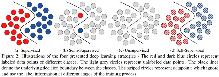
Illustrative learning setups from a 2020 classification survey.
Self-supervised learning differs from semi-supervised self-training. Self-training starts with a task model trained on labeled examples, uses that model to assign pseudo-labels to unlabeled examples, and retrains on selected predictions. SSL can construct its objective before any target-task model exists.
Four common self-supervised objective families
These families overlap. A method can mask an input, predict a latent target, and apply a contrastive loss in one training recipe.
1. Mask, denoise, and reconstruct
The pipeline hides or corrupts part of an observation, then asks the model to recover a token, pixel region, audio unit, or learned target. BERT masks text tokens. Masked Autoencoders reconstruct image patches. HuBERT predicts clustered units for masked speech frames.
The design choice is what to reconstruct. Pixel-level or waveform-level losses retain fine detail, including detail that may be irrelevant. Discrete or latent targets can focus the objective, but their quality depends on the tokenizer, clusterer, or teacher that produced them.
2. Predict context, order, or the future
These methods exploit spatial or temporal structure. Word2vec predicts words from their context. Causal language models predict the next token. Contrastive Predictive Coding (CPC) encodes a sequence and uses the current context to identify future latent segments among distractors.
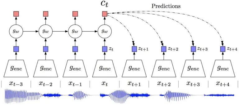
Audio CPC architecture from the 2018 Contrastive Predictive Coding paper.
Future prediction can force a model to preserve structure that remains stable over time. It can also over-reward local continuity. Evaluation must show that the learned features transfer to the intended task.
3. Align corresponding views with a contrastive objective
Contrastive methods bring positive pairs closer in representation space and separate selected negatives. In SimCLR, two augmentations of the same image form a positive pair. Views from other images in the batch act as negatives. CPC contrasts a true future representation with distractors.
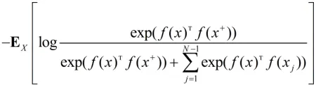
The InfoNCE objective used in Contrastive Predictive Coding.
The pairing policy defines the invariance. If two crops are declared equivalent, the representation learns to ignore their differences. That helps when the differences are nuisance variation and hurts when they carry the downstream label. Negative selection also matters because semantically similar examples can become false negatives.
4. Predict teacher or latent representations
Self-distillation methods train a student view to match a teacher representation. BYOL uses online and target networks without explicit negative pairs. DINO applies self-distillation to vision transformers. Latent-prediction methods such as I-JEPA predict the representation of a hidden image region from visible context instead of reconstructing every missing pixel.
These methods need mechanisms that prevent representation collapse, where many inputs map to nearly the same vector. Teacher updates, asymmetric branches, centering, normalization, variance constraints, or decorrelation can supply that pressure. The exact mechanism depends on the method.
Classic image pretext tasks from 2014 to 2018
Early visual SSL papers are still valuable teaching examples because the automatically generated target is easy to see. They are historical methods, not default recipes for every current vision system. Their shortcut controls also expose a durable lesson: a network will exploit any signal that reduces the loss, including signals the designer did not intend.
Spatial context and puzzles
The 2015 context-prediction task samples a central patch and a neighboring patch, then predicts the neighbor's relative position. Gaps, jitter, and color-channel changes make it harder to solve the task from boundaries or chromatic aberration alone.
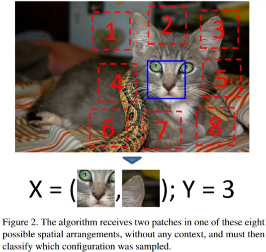
Relative patch prediction from Doersch et al., 2015.
The 2016 jigsaw task shuffles a grid of patches and asks a network to identify the permutation that restores their order. Sampling gaps and independent patch normalization limit low-level shortcuts.
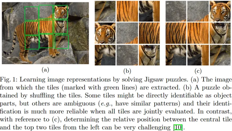
Jigsaw pretext task from Noroozi and Favaro, 2016.
A 2018 extension combined reordering, colorization, and missing-patch recovery in one damaged-puzzle task.
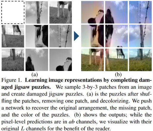
Damaged-jigsaw objective from Kim and colleagues, 2018.
Rotation and exemplar discrimination
RotNet rotates an image by 0, 90, 180, or 270 degrees and uses the known transform as the class label. The task can encourage object-sensitive features when images have a meaningful upright orientation. It is poorly matched to overhead, microscopic, or rotationally symmetric data.
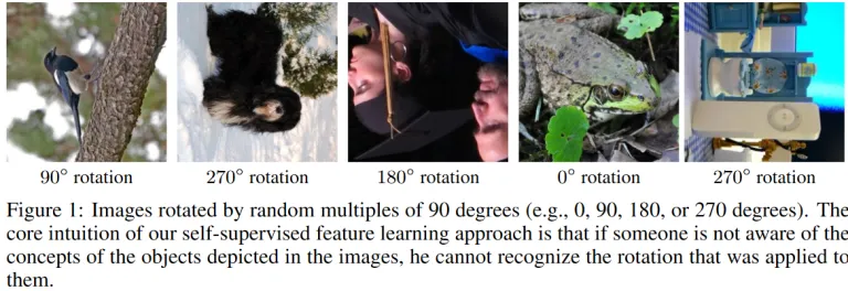
Rotation prediction from Gidaris et al., 2018.
Exemplar methods begin with an image patch, apply several transformations, and train the network to recognize transformed versions as the same instance. This line anticipated later view-matching objectives.
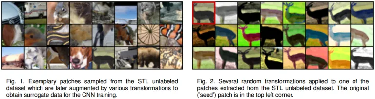
Exemplar transformations from Dosovitskiy and colleagues, 2014.
Inpainting and channel prediction
Context encoders remove an image region and train a network to fill it from surrounding pixels. The model must combine local texture with larger spatial context, although a plausible reconstruction does not prove that the representation is useful for every downstream task.
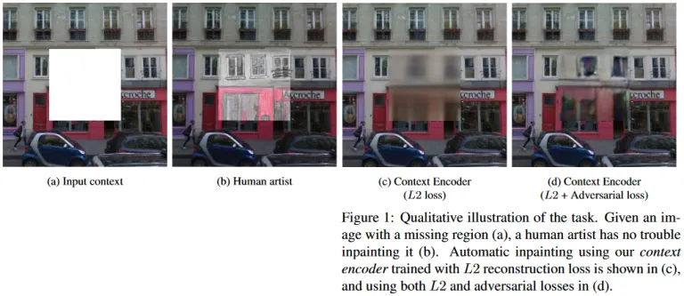
Image inpainting from Pathak and colleagues, 2016.
Colorization uses a grayscale image as input and the original color channels as targets. Split-brain autoencoders predict one subset of color channels from another in both directions.
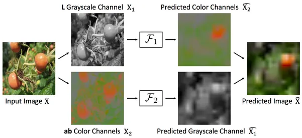
Cross-channel prediction from Zhang et al., 2017.
Motion and counting signals
Video provides temporal correspondence. A 2017 method used motion-based segmentation from video as a noisy supervisory signal for object features. A related video-colorization approach learned visual correspondence by propagating color between neighboring frames.
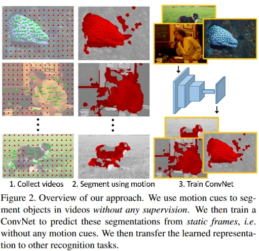
Motion-derived supervision from Pathak and colleagues, 2017.
Counting-based representation learning uses a consistency constraint: the predicted count for an image should equal the sum of predictions for non-overlapping parts. A second, unrelated image provides a contrastive case.
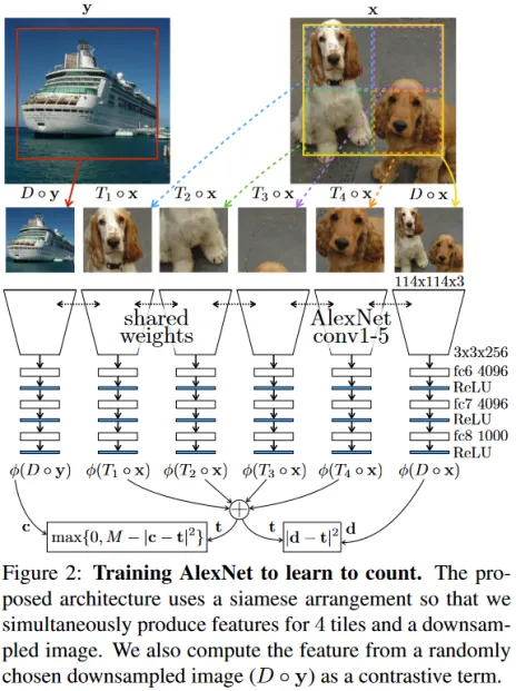
Counting consistency from Noroozi et al., 2017.
Clustering and multi-task training
DeepCluster alternates between clustering learned image features and treating cluster assignments as targets for representation updates. The targets change as the encoder changes. Multi-task self-supervised learning instead combines several pretext objectives under a shared trunk with task-specific heads.
These ideas survive in newer forms, but old benchmark claims should stay attached to their original datasets, architectures, and evaluation protocols. They are not timeless rankings.
Business examples: transactions and paired workplace signals
The useful business pattern is to find structure that operations already generate, then choose an objective that cannot be solved from a trivial field or timestamp. Transaction streams and synchronized sensor data provide two concrete examples.
Treat transaction sequences as a language-like stream
A transaction is an event with categorical fields such as merchant category code (MCC), channel, branch, product, or operation type, plus numerical values and time. A customer or account history becomes an ordered sequence of those events.
That structure supports several self-supervised objectives:
- Learn categorical embeddings from context. Treat an MCC or operation type like a token and nearby events like its context. The analogy comes from word2vec's skip-gram objective. Item2Vec applies the same idea to co-occurring items. For transactions, the context window must reflect the business process, and evaluation must show that proximity in the embedding space helps the actual downstream task.
- Recover masked fields or events. Hide one field, such as channel or MCC, and predict it from the remaining fields and surrounding events. A sequence model can also mask an entire event and recover its categorical values, amount band, or latent representation. VIME provides a related tabular pattern: corrupt feature values, then predict the mask and reconstruct the original data. Use a loss appropriate to each field type instead of forcing continuous amounts and categorical codes through one target.
- Predict transaction order. Swap adjacent events or shuffle a short window, then ask whether the order is valid or train the model to restore it. Temporal-order verification is an established self-supervised sequence objective, while CoLES shows a transaction-specific contrastive approach to event-sequence representations. Remove explicit ordering shortcuts from the corrupted example. If an untouched timestamp reveals the answer, the model learns the data pipeline rather than transaction dynamics.
Customer identifiers, post-event outcomes, and fields created after a decision can leak the downstream label. Build the pretraining record as if it were available at the downstream prediction time, then test embeddings on a temporally later split.
Use older or distribution-shifted records only under a documented protocol
Records excluded from supervised training because of age or distribution shift may still be candidates for representation pretraining. Age alone does not make them useful. Document why the records differ, including schema, product rules, customer population, channel, time period, and collection policy.
Keep the experiment bounded: pretrain the representation with and without the older records, adapt both versions on the same recent labeled set, and evaluate on a later representative window. Check performance by important subgroup as well as in aggregate. Retain the older corpus only when the transfer result holds and its use satisfies the approved data policy. A larger pretraining set can otherwise encode obsolete behavior, historical bias, or fields that no longer exist.
Use paired office video and audio as a cross-modal signal
Synchronized video and audio provide correspondence without a person labeling every frame. A model can predict an audio summary from a co-timed frame, decide whether clips align, or bring matching audio and visual embeddings together. The ambient-sound study is a foundational example of using sound associated with video frames to learn visual representations.
An office deployment needs a stricter data boundary than a research video corpus. Define the approved purpose, consent or other valid collection authority, notice, access, retention, deletion, and security controls before recording. Minimize identifiable speech and bystander capture rather than collecting them by default. Building layout, camera position, microphone response, occupancy patterns, and background machinery can all create domain shift, so separate evaluation by site and time period is necessary before using the representation in an operational task.
How to evaluate a self-supervised model
A lower pretraining loss only shows that the model optimized its constructed objective. It does not establish transfer quality. Use an evaluation plan that matches the real decision.
- Define the downstream tasks first. Include the task type and data conditions that matter in deployment. A vision encoder may need classification, retrieval, and dense prediction tests. A speech encoder may need word error rate, speaker verification, or noise robustness.
- State the adaptation protocol. A frozen k-nearest-neighbor test, a linear probe, few-label fine-tuning, and full fine-tuning answer different questions. Report which layers and parameters changed.
- Hold the comparison budget fixed. Record the pretraining data, model size, compute, augmentations, label budget, input resolution, optimization schedule, and downstream head. Protocol choices can change apparent rankings.
- Check leakage and overlap. Remove downstream test examples and near-duplicates from pretraining data where possible. For time-dependent applications, preserve a realistic temporal split.
- Measure robustness and subgroup behavior. Aggregate accuracy can hide failures by domain, speaker, language, capture device, or environment.
- Compare against a supervised baseline and no-pretraining baseline. SSL should justify its additional data and compute under the same downstream constraints.
A broad visual transfer study found that no evaluated self-supervised method dominated across all 40 downstream tasks. This is why a single linear-probe score cannot stand in for task-specific evaluation.
Common failure modes
| Failure mode | What goes wrong | Practical control |
|---|---|---|
| Shortcut learning | The model exploits borders, camera artifacts, timestamps, or other easy cues | Remove or randomize the cue, then test under distribution shift |
| Wrong invariance | An augmentation removes information the downstream task needs | Design views from task requirements and run ablations on each transform |
| False negatives or bad pairs | The loss pushes related examples apart or aligns unrelated observations | Audit pairing rules, use metadata carefully, and compare objectives with and without negatives |
| Representation collapse | Many inputs receive nearly identical embeddings | Monitor feature variance and covariance; use the method's anti-collapse mechanism |
| Domain mismatch | Large pretraining data differ from the deployment channel, language, or population | Add in-domain pretraining or adaptation and evaluate representative subgroups |
| Evaluation leakage | Pretraining contains test examples or close duplicates | Deduplicate across splits and document temporal and source boundaries |
| Hidden downstream label cost | Pretraining is label-free, while adaptation and acceptance tests still need annotation | Budget labels for fine-tuning, calibration, error analysis, and regression tests |
A practical decision rule
Self-supervised learning is a good candidate when you have abundant modality-native data, limited task labels, and a representation you expect to reuse. Its value is less clear when the available corpus is far from the deployment domain, labels are cheap, or the pretraining compute exceeds the value of better initialization.
Write a supervision ledger before training: list every data source, automatic target, pairing rule, human label, teacher model, and downstream adaptation step. Then evaluate the representation under the protocol the product will actually use.
For speech systems, that model-level decision sits inside a larger operational design. Continue with the voice AI infrastructure guide to map the speech model to media, runtime, tool, and observability requirements.