How our AI experts fought spoofing – and won

In a recent Voice Anti-spoofing Challenge hosted by ID R&D, participants were asked to develop an algorithm that can distinguish between human and spoofed voices. At Dasha AI, we’ve created a conversational AI with a special focus on speech recognition, so we couldn’t resist the temptation to give this challenge a shot. Together with his team, Stas Prikhodko, our ML Researcher and Kaggle expert, decided to join in  –  and won! In this article, Stas talks about state-of-the-art approaches to sound processing, as well as some of the setbacks and oddities he encountered during the competition.

There were only 98 participants, mostly because it was a sound processing challenge hosted on a Russian platform, and to top it all off, we had to run our solution in a Docker container. I teamed up with Dmitry Danevskiy, a Kaggle master who I’d met at another competition.

The task

We had to split 5 GB of audio files into spoof/human classes, predict their probabilities, wrap our solution in a Docker container and send it to the server. The solution needed to process the test data in 30 minutes and take up less than 100 MB.

The task description said that we needed to differentiate a person’s voice from an automatically generated one, although it seemed to me like the spoof class also included files where the sound was generated by bringing a loudspeaker up to the microphone (this is what spoofers do when they steal their victim’s voice recording for identification).

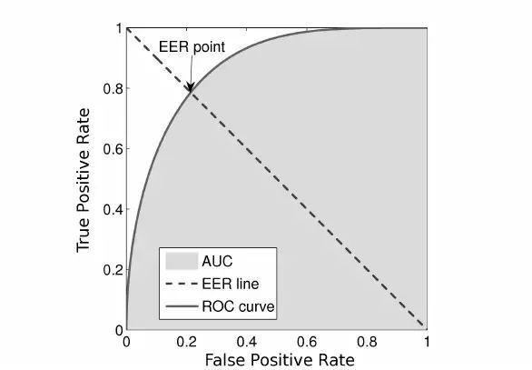
The proposed metric was EER:

We decided to use the first code we found onlinebecause the code provided by the contest organizers seemed too complicated.

The competition

The organizers introduced the baseline, which also happened to be the greatest riddle of the contest. The baseline seemed like a piece of cake: all we had to do was calculate the mel spectrograms, train a MobilenetV2 model and end up ranking 12th or lower.

You might be thinking there were only about a dozen people participating, but that wasn’t the case. All throughout the first stage of the contest, our team couldn’t cut through the baseline. Our code, which was ideally identical to the one suggested by the organizers, was showing considerably worse results. Any attempts to improve it (like switching to more complex neural networks or using OOF predictions) helped a little, but didn’t bring us closer to the baseline.

That was when something unexpected happened: about a week before the scheduled deadline, it turned out that the metric implementation had a bug and depended on the order of predictions. Around the same time, we also found out that the organizers hadn’t cut off internet access in Docker containers, so a lot of people downloaded the testing data.

When this surfaced, they put the contest on ice, uploaded the metric, refreshed the data, shut off the internet and ran the contest again for 2 more weeks. After the results had been recalculated, we were ranked 7th with one of our first submissions. Now it was clear we had to keep moving forward.

The model

We used a ResNet-like convolutional net trained on mel spectrograms.

1) There were five such blocks in total. After each block, we used deep supervision and increased the number of filters by 1.5.

2) During the competition, we switched from binary classification to multi-class in order to make the most of the mixup principle, which is basically mixing two sounds and summarizing their class labels. The switch also enabled us to artificially increase the probability of the spoof class by multiplying it by 1.3. This helped because we had a hunch that the class balance in the test set may be different from the training one, and this is how we improved the quality of the models.

3) We trained our models on folds and then averaged the predictions of several models.

4) We also made good use of Frequency Encoding. In a nutshell, 2D convolutions are position-invariant, so the output of a convolution would be the same no matter where the feature is located. Spectrograms are not images, the Y-axis corresponds to signal frequency, so it would be great to assist a model by providing this sort of information. To do so, we concatenated the spectrogram and matrix consisting of numbers in the interval from -1 to 1 from bottom to top.

To illustrate what I’m talking about, here’s the code:

n, d, h, w = x.size() vertical = torch.linspace(-1, 1, h).view(1, 1, -1, 1) vertical = vertical.repeat(n, 1, 1, w) x = torch.cat([x, vertical], dim=1)

5) We trained all this on the pseudo-label test data that had been leaked during the first stage as well.

Validation

Ever since the contest began, participants couldn’t seem to wrap their heads around the big question: why does local validation score 0.01 and lower in EER, the leaderboard scores 0.1, and the two don’t really correlate? We had two different hypotheses: either there were duplicates in the data, or the training data was collected on one set of speakers, and the test data on another.

The truth lied somewhere in between. It turned out that about 5% of the training set data was contained in duplicate hashes (in fact, there could also be different crops of the same file, but this wasn’t so easy to check, so we didn’t).

To test the second hypothesis, we trained a speaker-id network, got embeddings for each speaker, clustered them all using K-means, and applied K-fold cross-validation to the data. More specifically, we trained our models on speakers from one cluster, and predicted speakers from another. This validation method started to correlate with the leaderboard, although it also showed a score that was 3–4 times better.

Alternatively, we tried to validate only on predictions where the model was at least a little uncertain, meaning where the difference between the prediction and class label was > 10**-4 (0.0001), but this method didn’t prove useful.

So what went wrong?

It’s easy enough to find thousands of hours of human speech on the internet. Plus, a similar contest was already held several years ago. That’s why it seemed like an obvious idea to download a lot of data (we ended up with ~300 GB) and train the classifier using it. In some cases, training on such data slightly improved the final result if we trained on these additional and train sets before the plateau, and then used only the train data. However, with this method, the model converged in about 2 days, which meant 10 days for all the folds. That’s why we had to abandon this idea.

In addition, many participants noticed that the file length correlated with the class in the train set, but there was no sign of that in the test sample. The typical image networks like ResNeXt, NasNet-Mobile and MobileNetV3 weren’t of any great help.

Afterword

All the setbacks and hurdles I’ve mentioned didn’t stop us from winning the competition, and I’ll take full advantage of the experience to take sound processing to the next level here at Dasha AI. We’re always on the hunt for new challenges and knowledge. I hope you also learned something useful!

Finally, here’s our solution.