

Today you will learn about functions that "force" the algorithm to return the probabilities of attributes to classes. This blog post is designed for readers who have prior knowledge of this topic.
Let’s consider the problem of binary classification with classes {0, 1} in the case when the algorithm gives some estimate of a belonging to class 1. We can assume that the estimate lies on the interval [0, 1]. Ideally, it could be interpreted as an estimate of the probability belonging to class 1, but in practice, this is not always possible and this is exactly what I will cover in this post.
To assess the quality of the solution and adjust our algorithm, we use the L(y,a) error function. The error function is called proper scoring rules if:
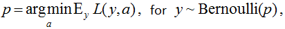
fig.1
i.e. the optimal answer for each object is the probability of its belonging to class 1.
Consider the Mean Squared Error (MSE; it is commonly used in regression, but in this case we will apply it in the classification problem), the error on an object is equal to the square of the deviation from the true label: SE=(y-a)2. If the object with probability p belongs to class 1, then the expected error is this:
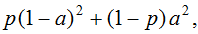
fig. 2
when minimizing it, we get (in essence, we take the derivative and equate to zero): a = p, i.e. SE is also an error scoring function. It is interesting that the minimum expectation value is:
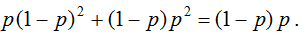
It coincides with the function that is optimized when constructing decision trees in the Gini impurity up to a multiplicative constant 2. The MSE function in classification problems is called the Brier score, and this is the name under which it is implemented in scikit-learn:

fig. 4
Choosing the splitting criterion among the two standard ones (entropy and Gini), you choose between the target functions for optimization. In various forums some say that the MSE cannot be used in classification tasks, yet it turns out that it can. Moreover, sometimes it is even preferable to logloss (we won’t argue here on what parameters as details can be found, for example, in this Selten's article). Although it must be said that the logistic error is the only scoring error in the class of local errors (local information about the distribution is used in the general case). In general, if you understand this topic, then it is easy to think of LS-GAN while looking at GAN (this is one of the first modifications that suggest itself for more effective training). To achieve this, one should delve into the fundamental areas of mathematics adjacent to ML, i.e. by replacing entropy / divergence (see examples below) with their analogs, you can get more effective solutions.
In a general scenario, in the theory of scoring functions in a problem with classes L = {1,2, ..., l}, when there is some true distribution of Q on L and the algorithm's answer is the distribution P, the following function is considered:
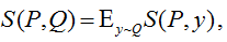
fig. 5
and is maximized by the first argument. Now consider the following function:
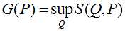
fig. 6
In this function, arguments are swapped for a reason. It is called an information measure or generalized entropy function. For example, for the Brier score, the generalized entropy, up to an additive constant, is equal to the quadratic entropy p12 +… + pl2. And the expression in fig. 7 is called divergence.
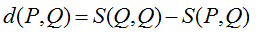
fig. 7
For the logistic error, this expression turns into the Kullback-Leibler divergence, and for the Brier score, it turns into the Euclidean distance.
Let's take a look at an example of a non-trivial scoring function. Let's replace the negation of the log in the logistic function with a very similar function:

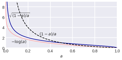
fig. 8
We obtain the following expression:
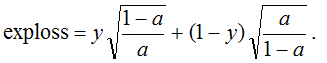
fig. 9
Let's carry out our standard procedure: we minimize the expected error for an object that belongs to class 1 with probability p:
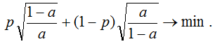
fig. 10
Taking the derivative and equating to zero, we obtain a = p, i.e. got one more error scoring function. The minimum expectation is as follows (i.e. the root of the minimum expectation when using ME):
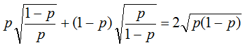
fig. 11 Let's justify the strange notation of exploss, the fact is that such an error function is called exponential, which is still strange since you can't see the exponent anywhere. In fact, the function is very logical for the following reason. Consider the problem of classification into two classes {–1, +1} and an algorithm for solving it, which gives some estimates of belonging to class 1 from the interval (–inf, + inf). The following error function seems to be very logical: exp (-a), which was used in the first variants of boosting. Its expectation on the object pexp(–a)+(1–p)exp(+a), and if we take the derivative and equate to zero, then we get:
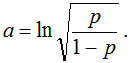
fig. 12
If we substitute this expression into the original error function, we will get just the exploss expression (only instead of the algorithm's answers there is a probability). Thus, this is the "natural correction" of the exponent if we want to interpret the responses of our algorithm as probabilities.
The technique when we receive the answer of some algorithm through the probability and then consider that our (already new) algorithm should give just this probability, is called the probability scale.
Not all error functions are scoring, but in general, there is a scoring criterion. The error scoring functions can be quite exotic, for example, the so-called Vince's crazy proper scoring rule: (1+y–a)exp(a).
Links:
Tilmann GNEITING, Adrian E. RAFTERY Strictly «Proper Scoring Rules, Prediction,and Estimation»
Matthew Parry, A. Philip Dawid and Steffen Lauritzen «Proper local scoring rules» The Annals of Statistics, 2012, Vol. 40, No. 1, 561–592
Barczy, M. (2020). A new example for a proper scoring rule. Communications in Statistics — Theory and Methods, 1–8. doi:10.1080/03610926.2020.1801737
Proper scoring rules: How should we evaluate probabilistic forecasts? (08.02.2019)