

Graph structures can naturally represent data in many emerging areas of AI and ML, such as image analysis, NLP, molecular biology, molecular chemistry, pattern recognition, and more.
Gori et al. (2005) first proposed a way to use research from the field of neural networks to process graph structure data directly, kicking off the field. Franco Scarselli et al. (2009) published a paper on the computational capabilities of GNNs. The strides were made in an attempt to solve the underlying difficulties of processing data represented on graphs and applying supervised or unsupervised learning algorithms to make predictions.
In today's article, you’ll get an introduction to graph neural networks. We’ll first review graph theory before looking at the difficulties of processing graphs along with graph prediction tasks in the first section. You’ll get to see areas where graphs are great for data visualization. The second section will build up on your knowledge with topics such as Node representation learning, graph augmentation, and graph processing problems.
Let’s get started:
Graph Theory - A Quick Refresher
Before looking at the graph neural network model, let's start with the basics by defining what a graph is.
A graph is basically a data structure made up of nodes and edges.
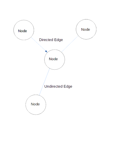
Nodes (or vertexes) contain information about entities. Edges (or links) represent the connections or relationships that exist between nodes. Links can also hold information, with attributes such as link identity or link weight. For instance, in molecular chemistry, links between atoms may represent different types of bonds such as covalent, ionic, metallic, hydrogen bonds, etc.
Edges may be directed or undirected. If a link is directed, it means that there is a defined direction from one source node to a destination node. Undirected edges don't have any semblance of destinations or sources, meaning that data can flow in all directions.
Graphs are described as existing in non-euclidean space. It essentially means that they can be represented in 3D unlike other data types such as text.
The structure of graphs can further be described as heterogeneous where nodes are of different types or homogeneous. Graphs may be static or dynamic, where vertexes and links change.
Dense graphs have many nodes and links, while sparse graphs are much simpler.
Graphs Are All Around Us
Graphs are all around us as fundamentally they represent relationships between entities. Images could very well be graphs, where each pixel may be a vertex connected to another node via a link. The nodes will contain a 3-dimensional RGB value showcasing the pixel information.
Text may also be thought of as a graph. A sentence will have several nodes (words) linked to each subsequent word to complete the sentence. In natural language processing, graphs may be used to showcase the relationships between words to help determine the meaning or context of a sentence.
Social networks may also be thought of as graphs. Interrelationships that exist between members of the network may be visualized, where entities are nodes and relationships are links.
Molecules have long been represented as graphs with nodes representing atoms and chemical bonds between atoms showcased as edges. You can consider using graphs in more applications for the following reasons:
They make it easier to deal with abstract concepts such as interactions, similarities, and relationships between entities;
Complex problems may be simplified and solved much more quickly by using graphs to create simplified representations.
Graph Prediction Tasks
There are three basic prediction problems when dealing with graphs: node-level, edge-level, and graph-level tasks. Let's look at what each entails:
Node-level
The task occurs at the node level with the aim of predicting the role or identity of the node within the graph. Zachary’s karate club is a classic example of node-level prediction analysis, where a conflict arises between the administrator and the instructor resulting in the 34 member club splitting into two factions. Based on the relationships and data about the members, the problem may entail predicting which faction each individual (node) may join based on the relationships (links) between them.
Node-level predictions may also be applied to other problems such as predicting parts of a speech or labeling pixels in an image. Supervised, unsupervised, or semi-supervised learning may be all applied to node-level tasks. Semi-supervised learning is the most commonly used method in node classification, as there is no need of labelling all the known nodes but the model can use associated information.
Edge Level
Edge-level prediction deals with predicting the probability of connectivity between node pairs in graphs, with models receiving prior training on the features of nodes and edges. The prediction model has caught the attention of various fields due to its wide applicability from predicting interactions in complex biological networks to being applied in establishing the relationship of drugs to diseases. It has also found success in identifying and establishing relationships between objects in images.
Graph Level
Graph level tasks deal with predicting the properties of entire graphs in graph generation. The core entails training a model on representative data, allowing it to generate graph-structured data. For instance, graph generation models based on GNNs have been previously used to discover new chemical structures and in drug design.
Difficulties of Using Graphs in Machine Learning
Some properties of graphs limit the possible actions and analysis that can be performed on them by machine learning models that prefer input in grid-like or rectangular arrays. Graphs can take on a range of sizes and structures. They also exist in non-euclidean space meaning that you can't use coordinates to represent the positions of nodes and edges. Graphs also lack a fixed form. If you try to convert a graph structure into its adjacency matrix, the resulting adjacency matrix may produce graphs of a wide range of appearances.
For instance, the same adjacency matrix can describe these two four-node graphs that look completely different visually and structurally.
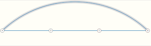
Aside from many adjacency matrices encoding the same connectivity, using the adjacency matrix can be further complicated if the number of edges is highly variable. Graphs are also permutation invariant, which means that changing the position and order of nodes may not have any effect on the results as long as the relationship between them remains the same. For instance, this may pose a problem in image analysis using data represented as a graph because changing the order of pixels may induce a difference in the image.
What is a Graph Neural Network?
Algorithm-based methods such as clustering, shortest path, spanning-tree, and searching algorithms have been the traditional way to approach graph analysis. They were limited as some prior knowledge of the graph needed to be gathered before applying the algorithms. Therefore, they did not provide any way to study the graph by itself or to perform graph-level classification.
Neural network graph theory differs as it's a deep-learning-based method that works on the graph domain with the ability to perform note classification, clustering, and link prediction. GNNs were introduced to solve the limitations of graph embedding and convolutional neural networks that lacked the ability to handle graph data. The need for GNNs also arose out of the growing accumulation of non-euclidean data that could be represented in graph form.
Now, what exactly is a graph neural network? In simple terms, it can be described as a machine-learning algorithm with the ability to extract information from graphs in a way that preserves the graph symmetries, including the nodes, edges, and global context. GNNs accept input in graph format and transform all the graph attributes to give an output without changing the connectivity or losing any topological information at the pre-treating stage.
At the core, GNN holds that nodes are defined by the information passed by neighbors. Every node has a state, and the goal is to learn the state embedding for each node. It entails learning about the node’s edge features and gathering information about neighboring nodes' states and features. State embedding is then used to arrive at an output.
There are different types of GNNs, including:
- Recurrent Graph Neural Network
- Graph Convolutional Network (GCN)
- Graph Auto-Encoder Network
- Gated Graph Neural Network
Each type may be better suited to individual problems. For instance, a gated graph neural network is applied for problems with long dependencies where gates are employed to remember information in previous states.
Graph Neural Network Applications
GNNs are able to solve several problems, including:
1. Node Classification
The problem involves trying to predict the labels of nodes by leveraging known labels or neighboring nodes. Semi-supervised learning may be used to train on node classification problems, where part of the graph is labeled, and part of it is not labeled. The model will then fill in the missing information. A real-world application in a social network may entail predicting the presence of bots masquerading as genuine users.
2. Clustering
Clustering entails trying to detect distinct structural groups in an existing graph. Graph clustering can be performed at a node level, where nodes may be grouped together based on similarities such as edge distances or weights.
3. Graph Classification
Entire graphs may be treated as objects and classified based on shared similarities. Graph classification may be utilized in many areas, such as NLP, to determine the semantic relationship between sentences treated as individual graphs.
4. Graph Visualisation
GNNs may be applied to visually represent data in graph form to reveal the structure and detect any animalities that may exist in the data.
5. Link prediction
Link prediction tasks deal with trying to decipher or predict if relationships exist between entities within a graph. An example of a real-world application may involve a recommendation model that attempts to show the most relevant products to users by predicting their preferences.
GNN Real-World Areas of Application
GNN’s have found many application areas as they have shown reliable performance in transforming graph input to a form that may be computed by learning algorithms without losing the actual dependence and connectivity. They have displayed a strong performance in facilitating the rapid processing of massive data, deep-level mining of topological information, and revealing the key features of data. Some popular areas of application include:
- Predicting the behaviors of chemical molecules;
- Deciphering relationships between words;
- Predicting document categories;
- Determining the relations of words and building syntactic relations in Natural Language Processing;
- Relationship prediction for objects detected from images in computer vision;
- Image generation from scene graph descriptions;
- Forecasting movements, volume, or density in traffic networks;
Challenges Affecting GNNs
While GNNs have proven to be better than CNNs at operating on non-euclidean data, there are still some challenges for the neural model. Scaling GNNs to large networks has been a persistent hurdle. The technology has faced more headwinds in handling dynamic graphs that keep changing and performing analysis of neural graph networks with many multiple layers.
Section Two
At this point, we assume that the reader now knows that a graph is a pair of sets of vertices (V) and edges (E), each edge is a pair of vertices, see Fig. 1.

Next, we’ll dive deeper into neural networks graph theory by first considering non-oriented graphs. That is, we assume that the edges are unordered two-element sets. Graphs arise in many analysis problems, especially when there are many objects and an obvious set of relationships between them (for example, a graph of users of a social network, in which each edge corresponds to the friendship between users).
Graph processing problem
Let’s first consider such a question: how to submit a graph to the input of a model (Fig. 3)? A conventional feed forward network (FFN) operates with a fixed input length, (fig. 2), therefore, the first option that comes to mind is to obtain a vector of a fixed dimension (representation or embedding) over the graph. We’ll get to that eventually. First, however, let’s note that there are other techniques for obtaining it, which I didn’t consider in this graph neural networks tutorial like random walks on the graph, for instance.


Another approach is the creation of special neural networks - "graph" (Graph neural networks or GNNs for short), which are capable of processing graphs. Note that an image is also a graph since it is not just a set of pixels, there are neighboring pixels for each pixel and this is important information, since their values, as a rule, are highly correlated, and their strong difference can mean the presence of contrast transitions in the image in the corresponding place: boundaries of objects. Fig. 4 shows examples of neighborhood graphs built using a matrix of pixels (these are the so-called 4- and 8-neighborhoods).
![]()
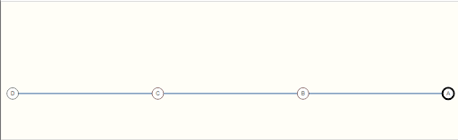
Text is also a graph, albeit a very simple one, because text is a finite set of words (and punctuation marks, which are sometimes neglected in analysis), on which linear order is introduced (there is the first word, the second, etc.), the corresponding graph is shown in Fig 5.

In the general case, an arbitrary graph can be very different from graphs that correspond to images and texts: it doesn’t have a clear structure, arbitrary degrees of vertices, etc. But still, we got some hints on how to process graphs using neural networks. In special cases, when a graph represents text or an image, such networks should be similar to classical ones for working with texts and images: convolutional, recurrent, transformers, etc.
Note that the order of vertices in a graph is often unimportant (as opposed to graphs of images and texts). Therefore, when processing graphs, the equivariance property is often crucial: if, for example, a network layer changes the labels of vertices, then when renumbering the vertices, the corresponding renumbering of labels occurs (as on fig. 5). In Fig 5 there are the two vertices that are indistinguishable from the point of view of the structure of the graph, so if you change their labels and pass through the graph network, then the response labels should also change.

That is why it is impossible to simply feed an adjacency matrix into an ordinary convolutional network: here the vertices are forcedly ordered, and the result of the convolutional layer is not equivariant with respect to the simultaneous identical permutation of rows and columns of such a matrix.
Node representation learning
First, we will consider a rather narrow task - node representation learning. In practice, we don’t have just a graph, each vertex (and / or edge) has a description (fig. 6); we will assume that this feature description is a real vector of fixed length. In the example with a social network about each user, we can know gender, age, etc. But such a representation doesn’t take into account information about the structure of the graph: it is local and doesn’t store information about the neighbors of the vertex (i.e., the user's friends).

GNNs compute vertex representations in an iterative process, different kinds of GNNs do that in different ways, and each iteration corresponds to a network layer. The simplest concept for such computation is Neural Message Passing. In general, Message Passing is a fairly well-known technique in graph analysis; each vertex has a certain state, which is refined in one iteration using the following formula:

hereinafter, N(v) is the neighborhood of the vertex v, AGG (AGGREGATE) is the aggregation function (in the sense, it collects information about neighbors, for example, summing their states), UPDATE is the function of updating the state of the vertex (taking into account the collected information about the neighbors). The only requirement imposed on the last two functions is differentiability, in order to use them in a computational graph and calculate the network parameters using the backpropagation method. The second function is sometimes also called COMBINE, since it takes into account both the current state of the vertex and the aggregation of its neighbors. Obviously, at one iteration, for each vertex, we use only information from its unit neighborhood - its “friends”, on the second, information from a second-order neighborhood (friends of friends) seeps into its updated representation, after the k-th iteration, from the neighborhood of k-th order.

In classical graph networks (original GNN, [1], [2]), the state change occurs according to a very simple formula:

that is, aggregation here is the usual summation, and when updating, the last state and the result of the aggregation are passed through linear layers (multiplied by matrices), then their linear combination with an offset is passed through the activation function.
One of the most popular graph networks is GraphSAGE (Graph Sample and Aggregate), and it has an almost identical formula:

vertical concatenation occurs in square brackets (the product of a matrix by concatenation corresponds to the sum of the products of matrices by concatenated vectors), but in the original work [3], different aggregations were used:
- Averaging - the mean,
- LSTM aggregation (using which neighbors were mixed),
- Pooling (line layer + pooling):

When using LSTM aggregation, the vertices from the neighborhood were ordered and the sequence of their representations was fed into the recurrent LSTM network. Added unsupervised loss to GraphSAGE (I won’t describe it in detail here, but the idea is that neighboring vertices get similar representations and random ones get dissimilar ones). Also, in the original publication ([3]), neighbors from the neighborhood were sampled (Fig. 8 shows an increase in the computation speed), the resulting state was normalized (but sometimes this is not done in the actual work).

Later, modifications of GraphSAGE were proposed, for example, PinSage [4], in which another sampling of the neighborhood states is performed (for processing large graphs), in particular, random walkings are made, sampling is performed among the top-k visited vertices, and the ReLU activation function is used. and the states of neighbors are passed through a separate module before aggregation.
In graph networks, the term self-loops means that we include it in the vicinity of a vertex and its state does not appear separately in the formula, for example, as here [5]:

Generalized Neighborhood Aggregation
More often, the aggregation was done by summing the states of neighbors, although you can use averaging (Neighborhood Normalization):

or

The latter averaging is used by Graph convolutional networks (GCNs). In [6], it was shown that it is important to choose the right aggregation, since it can lose some important information, for example, the degree of a vertex under ordinary averaging.
Another popular aggregation is set pooling [7]:

functions f and g are implemented by deep multi-layer perceptrons. Note that it has been proven that a network with such aggregation is a universal approximator.
Also, note Janossy pooling [8], in which the summation is performed over all permutations (this is in theory, but in practice - over several random ones).

The GIN (Graph Isomorphism Network) uses a fairly simple formula for state adaptation (and aggregation here is a simple summation) [9]:

There are Learnable Aggregators ([10]), and the simplest option is to include in the masking formula (vectors that are elementwise multiplied by the states of neighbors and are the outputs of a separate learning module):


And, of course, during aggregation, you can use the Attention, then the states of neighbors are summed up with attention coefficients:


Different attention mechanisms can be used, including those with several heads (we will not list them all); LeakyReLU was used as a function f in the original work on Neighborhood Attention: Graph Attention Network (GAT) [11]. The interpretation of the attention mechanism is present here: we look at our neighbors and then select the coefficients in the aggregation.
Adaptation problem
The main problem when using the described neural propagation of the so-called over-smoothing: after several iterations of vertex states recalculation, the representations of neighboring vertices become similar, since they have similar neighborhoods. To combat this, you can do the following:
use fewer layers of aggregation and more for "processing features", skip layers or concatenating states from previous layers, use architectures that have a memory effect (eg GRU).
For one of the methods of state concatenation in the theory of graph networks, there is the term "Jumping Knowledge Connections" [12]:

The DEEPGCNS network [13] also uses the idea of throwing as does DenseNet but the former also uses dilated convolutions by analogy, as is done in convolutional networks: the neighbors of the vertex are ordered and aggregation occurs by k of them, for ordinary convolution by the first k, for sparse with a step of 1: 1, 3, 5, etc. (fig. 10).
Graph aggregation
So far, we have considered ways to iteratively refine the representations of vertices, but we started with the fact that it would be nice to be able to represent a graph in the form of a fixed vector. How do you do this with vertex representations? The first obvious way is Graph Pooling, which is to summarize the views obtained:

Another approach is to consider that the set of vertices is a sequence, therefore, their representations can be fed to the input of the LSTM network, possibly with an attention mechanism. In the SortPool approach [14], the vertices are sorted (in some way, for example, by the last element in the vector-representation), the representations of the first k vertices are concatenated and fed to the input to an ordinary neural network.

There is also a group of approaches in which the graph is iteratively simplified. In fact, pooling in convolutional layers for images and texts just simplifies the graph, so in GNN it is also reasonable to have such an operation. In SAGPool (Self-Attention Graph Pooling) [15], the ratings-ratings of the vertices are iteratively obtained, leaving the top-vertices. The process continues until there is one left or to the Readout layer (this is done in the original publication). As the name suggests, SAGPool uses the attention mechanism.

Another method that uses graph simplification - DiffPool [16] - at each iteration, the graph vertices are clustered (in terms of the theory of graph networks - “community allocation”), the vertices are aggregated in clusters, we go to the graph with the vertices corresponding to the communities. In MinCutPool [17], clustering is performed by the spectral clustering method (k-means in a special space, which is obtained by finding the eigenvectors of the matrix obtained from the graph adjacency matrix).
Using GNN
Now let's consider what tasks and how are solved using graph networks. From what we currently know:
the input of the network is a graph, each vertex of which has a feature description. This description can be considered the initial state (representation) of the vertex (fig. 14), there may be layers that independently modify the views (for each vertex, its presentation is passed through a small network). (1 in fig. 14), there may be layers that modify the representations of all vertices, taking into account the representations of the neighboring vertices. (2 in fig. 14), there may be layers that simplify the graph (for example, reduce the number of vertices). (3) in fig. 14). there can be layers that receive a graph representation (a vector of fixed length) along with the current graph with vertex representations. (4 in fig. 14).

Typically, such networks are used for tasks:
node-level predictions, such as node classification, edge-level predictions, for example, in the problem of predicting the probability of occurrence of an edge in a graph (link prediction), graph-level predictions, for example for graph classification, community detection or relation prediction.
For the graph level predictions, a graph representation is taken (in pure form or passed through a feedforward network), the error function depends on the problem, for example, in the regression problem (a real number is determined from the graph), you can use such a formula:

In tasks at the vertex level, the same is done with the representations of the vertices:

in the tasks of clustering vertices (for example, community detection), clustering is carried out in the space of vertex representations. In tasks at the edge level, they work with the concatenation of the edge representation or with a function from a pair of representations, for example, with the dot product of representations:

Graph networks can also be used in tasks without labels, then in the error functions it is estimated how consistent the representations of the vertices and the graph containing these vertices are, for example, in Deep Graph Infomax (DGI), a discriminator is also used, which, for a pair (vertex representation, graph representation), tries to understand whether a vertex belongs to a graph, negative examples are obtained by modifying the original graph [18].
Graph Augmentation
As in other areas of deep learning, graph neural networks use augmentation - methods of increasing the training sample by modifying the initial data. In principle, the sampling of neighbors, which we considered, in a sense, changes the original information. If the graph is sparse, then it is replenished with edges according to the principle "my friend's friend is my friend." If dense and large, then in some problems subgraphs are taken.
What have we not covered?
The most important questions that we have not yet touched on:
application of spectral graph theory in graph networks, including obtaining representations of convolutions, other robust graph analysis methods, generative graph networks, examples of graph network applications and libraries for GNN implementation.
Links
There is some good reading material on graph networks. First of all, here are some great review books:
- Hamilton «Graph Representation Learning» https://www.cs.mcgill.ca/~wlh/grl_book/files/GRL_Book.pdf
- Zhiyuan Liu, Jie Zhou «Introduction to Graph Neural Networks» // 2020
Secondly, a bunch of good reviews came out recently. A lot of information in this post came from these:
- Understanding Convolutions on Graphs https://distill.pub/2021/understanding-gnns/
- A Gentle Introduction to Graph Neural Networks https://distill.pub/2021/gnn-intro/
References
[1] Merkwirth, Christian & Lengauer, Thomas «Automatic Generation of Complementary Descriptors with Molecular Graph Networks». Journal of chemical information and modeling, 2005. 45. 1159-68. https://www.researchgate.net/publication/7583033_Automatic_Generation_of_Complementary_Descriptors_with_Molecular_Graph_Networks [2] F. Scarselli, M. Gori, A. C. Tsoi, M. Hagenbuchner and G. Monfardini, "The Graph Neural Network Model," in IEEE Transactions on Neural Networks, vol. 20, no. 1, pp. 61-80, Jan. 2009, doi: 10.1109/TNN.2008.2005605. https://ieeexplore.ieee.org/document/4700287 [3] W. L. Hamilton, R. Ying и J. Leskovec «Inductive Representation Learning onLarge Graphs» // https://arxiv.org/pdf/1706.02216.pdf [4] R. Ying, R. He, K. Chen, P. Eksombatchai, W. L. Hamilton, and J. Leskovec. 2018a. Graph convolutional neural networks for web-scale recommender systems. In Proc. of SIGKDD. DOI: 10.1145/3219819.3219890 [5] George T. Cantwell, M. E. J. Newman «Message passing on networks with loops» // https://arxiv.org/abs/1907.08252 [6] Thomas N Kipf, Max Welling «Semi-supervised classification with graph convolutional networks» // ICLR, 2017. [7] M. Zaheer, S. Kottur, S. Ravanbakhsh, B. Poczos, R. R. Salakhutdinov, and A. J. Smola. 2017. Deep sets. In Proc. of NIPS, pages 3391–3401. https://arxiv.org/pdf/1703.06114.pdf [8] Ryan L. Murphy «Janossy pooling: learning deep permutation-invariant functions for variable-size inputs» // https://arxiv.org/pdf/1811.01900.pdf [9] K. Xu и др. «How Powerful are Graph Neural Networks?» // https://arxiv.org/pdf/1810.00826.pdf [10] Z. Li и H. Lu. «Learnable Aggregator for GCN» // https://grlearning.github.io/papers/134.pdf [11] P. Velickovic, G. Cucurull, A. Casanova, A. Romero, P. Lio, and Y. Bengio «Graph attention networks» // In Proc. of ICLR, 2018 [12] K. Xu, C. Li, Y. Tian, T. Sonobe, K. Kawarabayashi, and S. Jegelka. 2018. Representation learning on graphs with jumping knowledge networks. In Proc. of ICML, pages 5449–5458. https://arxiv.org/pdf/1806.03536.pdf [13] G. Li, M. Muller, A. Thabet, and B. Ghanem «DeepGCNs: Can GCNs go as deep as CNNs?» // In Proc. of ICCV 2019 [13b] Cangea, C., Velickovic, P., Jovanovic, N., Kipf, T., and Lio,P. «Towards sparse hierarchical graph classifiers» // arXiv:1811.01287, 2018. [14] M. Zhang, Z. Cui, M. Neumann, Y. Chen «An End-to-End Deep Learning Architecture for Graph Classification» [15] J. Lee, I. Lee, J. Kang «Self-Attention Graph Pooling» [16] R. Ying и др. «Hierarchical Graph Representation Learning with Differentiable Pooling» // https://arxiv.org/pdf/1806.08804.pdf [17] Filippo Maria Bianchi «Spectral Clustering with Graph Neural Networks for Graph Pooling» // https://arxiv.org/pdf/1907.00481.pdf [18] Petar Veličković, William Fedus, William L. Hamilton, Pietro Liò, Yoshua Bengio, R Devon Hjelm «Deep Graph Infomax» // https://arxiv.org/abs/1809.10341