Binary classification quality functionals

Let’s consider a problem of classification into two classes (labeled 0 and 1), fig. 1 shows its graphical representation.

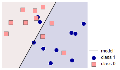
fig. 1 Illustration of the problem with two classes and a possible solution.

Let the classifier output the class label. We will use the following notation: yi is the label of the i-th object, ai is the answer on this object, m is the number of objects in the sample.

A natural, simple and common model metric is Accuracy (or Mean Consequential Error):

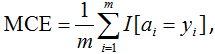
fig. 2

i.e. it’s simply the proportion (percentage) of objects for which the algorithm gave correct answers. The disadvantage of this functionality is obvious: it is bad in case of class imbalance when there are significantly more representatives of one class than the other. In this case, from a precision point of view, it is almost always advantageous to issue the label of the most popular class. Yet it may not be consistent with the logic of using the solution to the problem. For example, in the task of detecting a very rare disease, an algorithm that classifies everyone as "healthy" would not be useful.

Now let’s take a look at the confusion matrix - a 2×2 matrix, the ij-th position of which is equal to the number of objects of the i-th class, to which the algorithm has assigned the label of the j-th class.

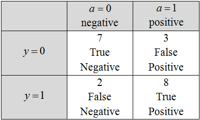
fig. 3 Confusion matrix

Fig. 3 shows such a matrix for solving for fig. 1, the names of the matrix elements are also shown here. The two classes are classified as positive (usually labeled as 1) and negative (usually labeled as 0 or –1). Objects that the algorithm classifies as positive are called Positive, those that actually belong to this class are True Positive, and the rest are False Positive. There is a similar terminology for the Negative class. We can use the following abbreviations:

TP = True Positive,

TN = True Negative,

FP = False Positive,

FN = False Negative.

Note: sometimes the error matrix is depicted differently - in a transposed form (the algorithm answers correspond to rows, and the correct labels correspond to columns).

Note: standard terminology is a little illogical: it is natural to call objects of a positive class as positive objects, but here objects assigned by the algorithm to a positive class (i.e., this is not even a property of objects, but of an algorithm). However in the context of using the terms "true positive" and "false positive", this already seems logical.

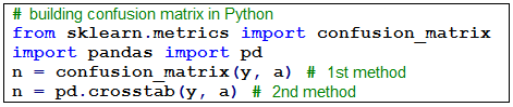
fig. 4 Accuracy is calculated with the following formula:

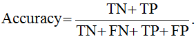
fig. 5

Classifier errors are divided into two groups: the first and the second type. Ideally (when the accuracy is 100%) the disparity matrix is diagonal, errors cause two off-diagonal elements to differ from zero:

Type I Error occurs when an object is erroneously classified as a positive class (= FP/m).

Type II Error occurs when an object is erroneously classified as a negative class (= FN/m).

The header image shows a well-known comic illustration of type 1 and type 2 errors: type 1 error (left) and type 2 error (right). When I explain to students, I always give an example that allows them to remember the difference between errors of type 1 and 2. Let’s say, a student shows up to an exam. If he studied the material and knows it well, then he belongs to the class with the label 1, otherwise, he belongs to the class with the label 0 (it is quite logical to call the knowledgeable student "positive"). Let the examiner play the role of a classifier: put a pass (i.e., mark 1) or send for a make-up exam (mark 0). The most desirable for a student "did not learn anything, but passed" corresponds to an error of the 1st type, the second possible error "learned the material, but did not pass" corresponds to the 2nd type.

The following functions are expressed through the notation introduced above:

Sensitivity (True Positive Rate, Recall, Hit Rate) reflects what percentage of objects of a positive class we correctly classified:

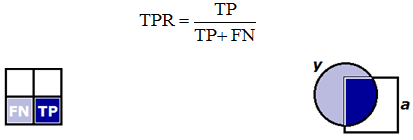
fig. 6

Here and below, the numerator of the formula (in dark blue) and the denominator (in dark and light blue) are shown. On the left, this is done for the inconsistency matrix, on the right - for sets: round - objects of a positive class, square - positive objects according to the classifier.

Precision (Positive Predictive Value) reflects what percentage of positive objects (i.e. those that we consider positive) are correctly classified:

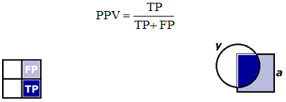
fig. 7

Precision and sensitivity can informally be called “orthogonal metrics”. It is easy to construct an algorithm with 100% sensitivity: it assigns all objects to class 1, but the precision can be very low. It isn’t difficult to construct an algorithm with precision close to 100%: it classifies only those objects in which it’s certain about to class 1, yet the sensitivity might be low.

F1 score is the harmonic mean of precision and sensitivity, which maximizes this functional leads to simultaneous maximization of these two "orthogonal metrics":

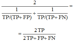
fig. 8

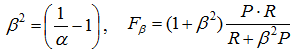
It’s also necessary to look at the weighted harmonic mean of precision (P) and recall (R) - Fβ score:

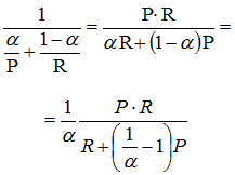
fig. 9

Note that β here is not a weight in harmonic mean:

The reason why the harmonic mean is used is clear from fig. 11, which show the level lines of the various averaging functions.

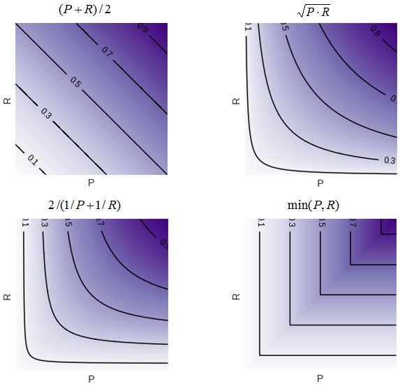
fig. 11 Level lines of some functions of two variables (in the first quadrant).

It can be seen that the lines of the harmonic mean level are very similar to the "corners", i.e. similar to the line of the min function, which forces a smaller value to “pull up” when maximizing the functional. If, for example, the precision is very small, then an increase in the sensitivity, even if by a factor of two, does not greatly change the value of the functional. This is shown more clearly in fig. 12: with 10% precision, the F1-measure cannot be more than 20%.

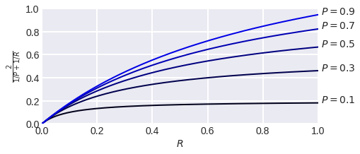
fig. 12 Dependence of F1 measure on sensitivity at fixed precision.

When using the Fβ measure, the level lines are "skewed", one of the metric (precision or sensitivity) becomes more important during optimization (fig. 13).

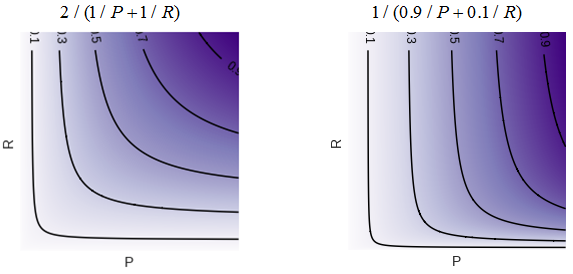
fig. 13 F measure and F1/3 measure level lines.

Among the quality functionals that are obtained from the inconsistency matrix, you can also note Specificity or TNR - True Negative Rate:

fig. 14 i.e. percentage of correctly classified objects of the negative class. As mentioned above, TPR is sometimes called Sensitivity and is used in conjunction with specificity to assess quality, and these two are often averaged (more on this later). Both functions have the meaning of "the percentage of correctly classified objects of one of the class." We can introduce the notion of Rk TPR for the k-th class: this is TPR, if the class k is considered positive, and then we can regard the following:

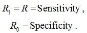
fig.15

Let’s also remember the False Positive Rate (FPR, fall-out, false alarm rate):

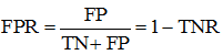
fig. 16

•  the proportion of objects of a negative class, which we mistakenly referred to as positive (this is necessary to understand the AUC ROC functionality).

MCC – Matthews Correlation Coefficient is

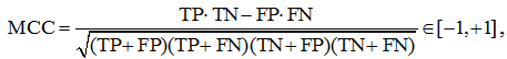
fig. 17

and it is recommended to be used for unbalanced samples. 

Let's see what this "complex formula" means. Consider the geometric mean of precision and TPR:

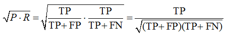
fig. 18

Let’s take the geometric mean of the precision and TPR of class 0 (i.e., assuming this class to be positive), by multiplying these geometric means we get the following:

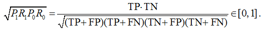
fig. 19

It is logical to maximize the resulting formula; by analogy, you can write out a formula for minimization. If we now look closely at the MCC formula, it becomes clear what it means and why its value lies on the segment [–1, +1].

Cohen’s Kappa

In classification problems, Cohen's Kappa quality functional is often used. Its idea is quite simple: since the use of Accuracy raises doubts in problems with a strong class imbalance, its values should be renormalized a little. This is done using the chance adjusted index statistics: we will normalize the accuracy of our solution using the accuracy that could be obtained by chance (Accuracychance). By chance here we mean the accuracy of the solution, which is obtained from our random permutation of answers.

fig. 20

The probability of guessing class 0 is highlighted in red, and class 1 is highlighted in blue. Indeed, the class k is guessed if the algorithm outputs the label k and the object really belongs to this class. We will assume that these are independent events (we want to calculate the random precision). The probability of belonging to class k can be estimated by confusion matrix as the proportion of objects of class k. Similarly, we estimate the probability of issuing a label as the proportion of such labels in the responses of the constructed algorithm.

Balanced Accuracy

In the case of class imbalance, there is a special analog of accuracy - balanced accuracy:

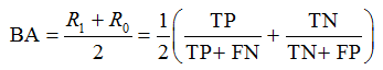
fig. 21

In order to make memorization easier, this is the average of TPR of all classes (we will come back to this definition in a bit), or in other terms: the average of Sensitivity and Specificity. Note that sensitivity and specificity are also, informally speaking, “orthogonal metrics”. It is easy to make the specificity 100% by assigning all objects to class 0, while there will be 0% sensitivity, and vice versa, and if all objects are assigned to class 1, then there will be 0% specificity and 100% sensitivity.

If in the binary problem of classifying the representatives of two classes approximately equal, then TP + FN ≈ TN + FP ≈ m/2 and the balanced accuracy is approximately equal to accuracy.

All of these functionals are implemented in the scikit-learn library:

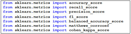
fig. 22

Comparison of functionals

Consider a model problem in which the distribution densities of the classes on the estimates generated by the algorithm are linear (fig. 23). The algorithm gives estimates of belonging to class 1 from the segment [0, 1] and it’s on this very segment that they are linear. Fig. 23 shows a finite small sample that corresponds to the depicted densities, but we will assume that the sample is infinite, since the densities are simple and allow us to explicitly calculate the quality functionals even in the case of such an infinite sample. We will assume that the classes are equally probable, i.e. our endless sample is balanced. The selected problem is very convenient for research and has already been used in the analysis of the AUC ROC functional.

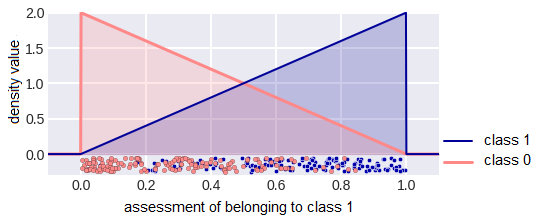
fig. 23 Distribution densities of classes in a model classification problem

Note that similar distributions arise in the problem shown in fig. 24 (the objects lie inside the square [0,1] × [0,1], the two classes are separated by the diagonal of the square) if the algorithm gives the values of the first feature as an estimate.

fig. 24 Representation of the model problem in the feature space

By depicting the densities a little differently, we can explicitly calculate the elements of the confusion matrix at a specific binarization threshold (fig. 25). All of them are proportional to the areas of the selected zones (note the scale of the axes):

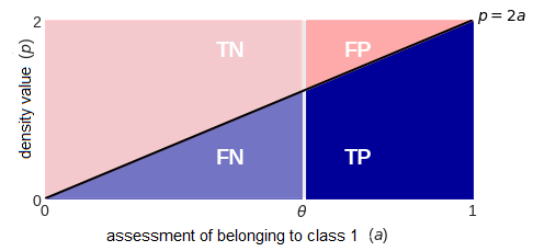
fig. 25 Convenient representation of densities: crossing the line drawing a = θ, we get the density values in the form of the lengths of the segments that fall on the corresponding colored zones: blue - for class 1, pink - for class 0.

We can now derive formulas for the considered quality functionals as a function of the binarization threshold:

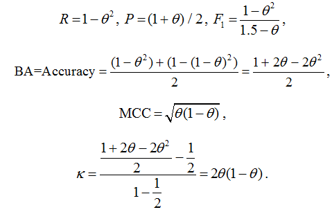
fig. 26 

Try to derive these formulas yourself, in addition, try to determine the binarization thresholds at which the specified functionals are maximal (you will encounter a surprise here).

A question arises here: in practice, we don’t have infinite samples, so what will change if we calculate the values of the functionals on a finite one, whose objects are generated in accordance with the indicated distributions? Part of the answer to this question is shown in fig. 27. As you can see, the curves are quite close to the theoretical ones at m=300; when the sample is increased by 10 times, they practically coincide.

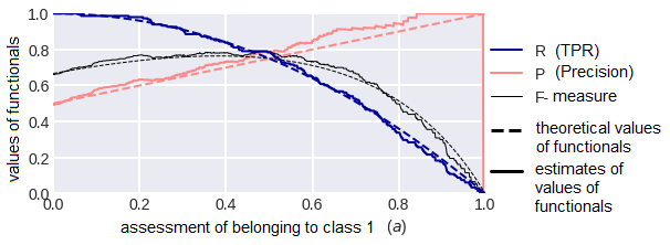
fig. 27

Let’s consider the graphs of our quality functionals as functions of the binarization threshold (fig. 28). Note that apart from the F1-measure, they are all symmetric with respect to the threshold 0.5, and this is quite logical. Now let's consider the situation of unequal classes, i.e. when the sample is unbalanced. Fig. 29 shows the graphs of functionals in the case when class 1 is twice as common in the sample as class 0. Note that all graphs have become asymmetric, except for the balanced precision graph - this function does not depend on the proportions of the classes!

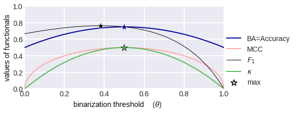
fig.28 Metrics as functions of the binarization threshold.

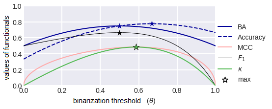
fig. 29 Metrics as a function of the binarization threshold for class imbalance (class 1 is twice as likely as class 0).