Let’s start with the basics. AUC ROC stands for the area under a receiver operating characteristic. The area under the ROC curve is one of the most popular quality functionals in binary classification problems. In my opinion, there are no simple and complete sources of information on "what is this?". As a rule, the explanation begins with the introduction of different terms (FPR, TPR), which a normal person immediately forgets. Also, there is no analysis of any specific tasks for the ROC AUC. This post describes how I explain this topic to students and my staff. We will discuss how to calculate ROC and will be calculating AUC formula (and by that I mean the formula for the computation of the area under the curve).
AUC = area under curve; ROC = receiver operating characteristic
Now, what do ROC and AUC stand for? ROC (sometimes called the "error curve") stands for receiver operating characteristic (ROC curve), AUC stands for “area under the ROC curve”.
Suppose a classification problem with two classes {0, 1} is being solved. The algorithm gives some estimate (and, perhaps, the probability) of an object belonging to class 1. We can assume that the estimate belongs to the segment [0, 1].
Often, the result of the algorithm's operation on a fixed test sample is visualized using the ROC curve (ROC = receiver operating characteristic, sometimes called the "error curve"; roc curve auc), and the quality is assessed as the area under this curve - AUC (AUC = area under the curve). Let's show with a specific example how the curve is constructed.
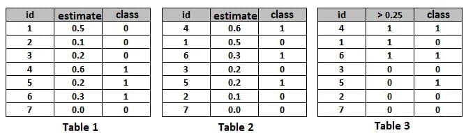
Let the algorithm give estimates as shown in table. 1. Let's arrange the rows of Table 1 in descending order of the algorithm's answers - we will get Table 2. It is clear that, ideally, its “class” column will also become ordered (first there are 1, then 0); in the worst case, the order will be reversed (first 0, then 1); in the case of "blind guessing" there will be a random distribution of 0 and 1.
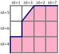
To draw a ROC curve, you need to take a unit square on the coordinate plane (as shown in fig.1), divide it into m equal parts by horizontal lines and into n by vertical lines, where m is the number 1 among the correct test marks (in our example, m=3), n is the number of zeros (n=4). As a result, the square is divided by a grid into m×n blocks.
Now we will look through the rows of Table 2 from top to bottom and draw lines on the grid, passing them from one node to another. We start from (0, 0). If the value of the class label in the viewed line is 1, then we take a step up; if 0, then we take a step to the right. It is clear that in the end, we will get to the point (1,1) because we’ll take a total of m steps up and n steps to the right.
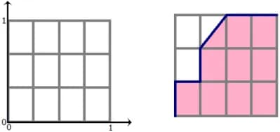
Fig. 1 (on the right) shows the path for our example - this is the ROC curve. Note: if several objects have the same rating values, then we take a step to a point that is a blocks higher and b blocks to the right, where a is the number of ones in the group of objects with one label value, and b is the number of zeros in it. In particular, if all objects have the same label, then we immediately step from point (0,0) to point (1,1).
ROC AUC is the area under the ROC curve and is often used to evaluate the ordering quality of two classes of objects by an algorithm. It is clear that this value lies in the [0,1] segment. In our example, ROC AUC value = 9.5/12 ~ 0.79.
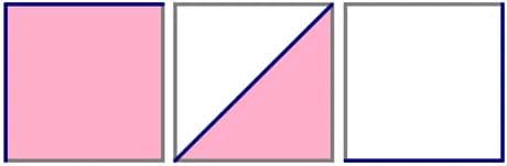
Above, we described the cases of ideal, worst, and random label sequence in an ordered table. The ideal corresponds to the ROC AUC-curve passing through the point (0,1), the area under it equals 1. The worst is the ROC-curve passing through the point (1,0), the area under it is 0. Random label sequence is something similar to the diagonal square and the area approximately equals 0.5.
Note: The ROC curve is considered undefined for a test sample consisting entirely of objects of only one class. Most modern implementations throw an error when trying to build it in this case.
The meaning of ROC AUC
The grid in fig. 1 divided the square into m×n blocks. Exactly the same number of pairs of the form (object of class 1, object of class 0), composed of objects of the test sample. Each shaded block in fig. 1 corresponds to a pair (object of class 1, object of class 0), for which our algorithm correctly predicted the order (an object of class 1 received a score higher than an object of class 0), an open block corresponds to a pair on which it made a mistake.
Thus, the area under the curve is equal to the fraction of pairs of objects of the form (object of class 1, object of class 0), which the algorithm ordered correctly, i.e. the first object comes first in the ordered list. Numerically, this can be written as follows:
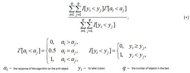
Note: In the formula (*), everyone is constantly mistaken, forgetting the case of equality of the algorithm's answers on several objects. Also, everyone is constantly rediscovering this formula. It is good because it can be easily generalized to other tasks of teaching with a teacher.
ROC Decision Making
So far, our algorithm has been giving estimates of belonging to class 1. It’s clear that in practice we often have to decide which objects belong to class 1 and which belong to class 0. To do this, it’ll be necessary to choose a certain threshold (objects with estimates above the threshold are considered to belong to class 1, others - to class 0).
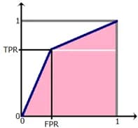
The selection of the threshold corresponds to the selection of a point on the ROC AUC curve. For example, for a threshold of 0.25 and for our example the point is shown in fig. 4 (1/4, 2/3) (take a look at table 3).
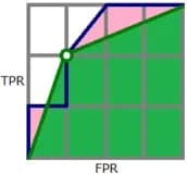
Note that 1/4 is the percentage of class 0 points that are incorrectly classified by our algorithm (this is called FPR = False Positive Rate), 2/3 is the percentage of class 1 points that are correctly classified by our algorithm (this is called TPR = True Positive Rate ). It is in these coordinates (FPR, TPR) that the ROC curve is plotted. It is often defined in the literature as the curve of TPR versus FPR with a varying threshold for binarization.
By the way, for binary answers of the algorithm, you can also calculate the AUC ROC, although this is almost never done, since the ROC curve consists of three points connected by lines: (0,0), (FPR, TPR), (1, 1), where FPR and TPR correspond to any threshold from the interval (0, 1). In fig. 4 (green) shows the ROC curve of the binarized solution, note that the AUC value after binarization decreased and became equal to 8.5 / 12 ~ 0.71.
In the general case, as can be seen from fig. 5, AUC ROC for a binary solution is as follows:

(as the sum of the areas of two triangles and a square). This expression has an independent value and is considered "honest accuracy" in a problem with an imbalance of classes.
A model problem
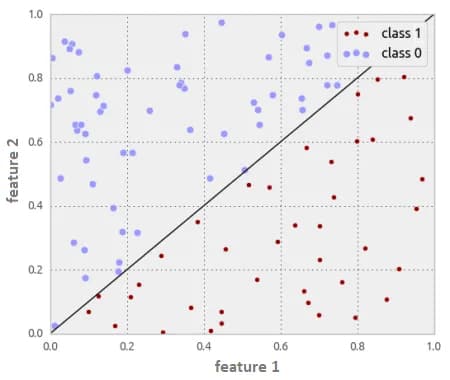
In the responses of the algorithm a(x), objects of class 0 are distributed with p(a) = 2-2a density, and objects of class 1 are distributed with p(a) = 2a density, as shown in fig. 6. It’s intuitively clear that the algorithm has some separating ability (most objects of class 0 have a score less than 0.5, and most objects of class 1 have a higher one). Try to guess what the ROC AUC is here, and we'll show you how to build a ROC curve and calculate the area under it. Note that here we are not working with a specific test sample, but we believe that we know the distributions of objects of all classes. This can be, for example, in a model problem, when objects lie in the unit square, objects above one of the diagonals belong to class 0, the objects below belong to class 1, logistic regression is used to solve it (as in fig. 7). In the case when the solution depends only on one feature (for the second, the coefficient is zero), we get exactly what was just described in our problem.
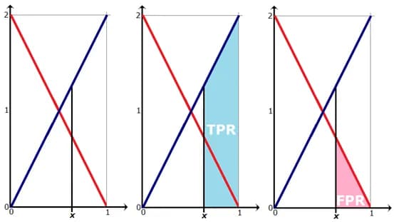
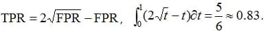
The TPR value when choosing the binarization threshold is equal to the area shown in fig. 6 (center), and FPR is the area shown in fig. 6 (right), and we get the following:

The parametric equation for the ROC curve is obtained, you can immediately calculate the area under it:
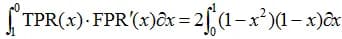
But if you don't like parametric notation, it's easy to do the following:
Note that the maximum accuracy is achieved at a binarization threshold of 0.5, and it is 3/4 = 0.75 (which does not seem very large). This is a common situation: the AUC ROC curve is significantly higher than the maximum achievable accuracy!
By the way, the AUC ROC curve of the binarized solution (at the binarization threshold of 0.5) is 0.75.
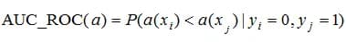
In such a “continuous” formulation of the problem, when objects of two classes are described by densities, it has a probabilistic meaning: it is the probability that a randomly taken object of class 1 has a class 1 rating higher than a randomly taken object of class 0.
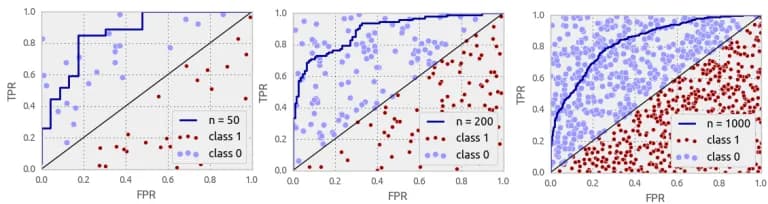
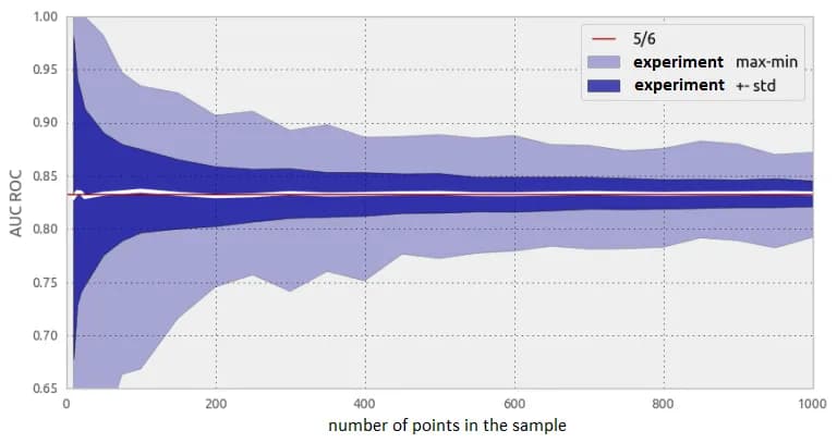
For our model problem, several experiments can be carried out: take finite samples of different cardinality with the indicated distributions. Fig. 8 shows the ROC AUC values in such experiments: they are all distributed around the theoretical value of 5/6, but the spread is large enough for small samples. Remember: the sample of several hundred objects is small to estimate the ROC AUC!
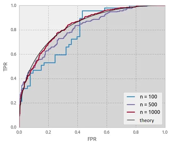
It is also helpful to see what the ROC curves look like in our experiments. Naturally, as the sample size increases, the ROC curves drawn from the samples will converge to the theoretical curve (plotted for the distributions).
Note:
Interestingly, in the considered problem, the initial data are linear (for example, the densities are linear functions), and the answer (ROC-curve) is a non-linear (and even non-polynomial) function.
Note:
For some reason, many believe that the ROC curve is always a step function - only when it is built for a finite sample, in which there are no objects with the same estimates.
Maximizing ROC AUC in practice
It’s difficult to directly optimize it for several reasons:
- this function is not differentiable by the parameters of the algorithm,
- it’s not explicitly split into separate terms that depend on the answer on only one object (as happens in the case of log_loss).
There are several approaches to optimization
- replacement in (*) of the indicator function by a similar differentiable function,
- using the meaning of the functional (if this is the probability of correct ordering of a pair of objects, then you can go to a new sample consisting of pairs),
- ensemble of several algorithms with the conversion of their ratings into ranks (the logic here is simple: AUC ROC depends only on the order of objects, therefore, specific ratings should not significantly affect the answer).
Notes
- ROC AUC does not depend on strictly increasing transformation of the algorithm responses (for example, squaring), since it does not depend on the responses themselves, but on the object class labels when ordering by these responses.
- AUC vs ROC not considered here.
- The Gini quality criterion is often used, it takes a value on the interval [–1, +1] and is linearly expressed through the area under the error curve:
Gini = 2 ×AUC_ROC – 1
- The AUC-ROC can be used to assess the quality of features. We believe that the values of the feature are the answers of our algorithm (they do not have to be normalized to the segment [0, 1], because the order is important to us). Then the expression 2 × | AUC_ROC - 0.5 | is quite suitable for assessing the quality of a feature: it is maximum if the 2 classes are strictly separated according to this feature and minimum if they are "mixed".
- Almost all sources provide an incorrect algorithm for constructing the ROC curve and calculating the AUC ROC curve. According to our description, these algorithms are easy to fix.
- It is often argued that the ROC AUC is unsuitable for problems with severe class imbalance. At the same time, completely incorrect justifications for this are given. Let's consider one of them. Let there be 1,000,000 objects in the problem, with only 10 objects from the first class. Let's say that the objects are websites, and the first class is the websites relevant to a certain query. Consider an algorithm that ranks all websites according to this query. Let him put 100 objects of class 0 at the beginning of the list, then 10 objects of class 1, then all the rest of class 0. AUC ROC will be quite high: 0.9999. At the same time, the answer of the algorithm (if, for example, this is a search engine output) cannot be considered good: there are 100 irrelevant sites at the top of the search results. Of course, we will not have the patience to scroll through the results and get to the 10 most relevant ones. What do you think is wrong with this example? The main thing is that it does not use the class imbalance in any way. With the same success, objects of class 1 could have been 500,000 - exactly half, then the AUC ROC is slightly smaller: 0.9998, but the point remains the same. Thus, this example does not show the inapplicability of AUC ROC in problems with class imbalance, but only in search problems. There are other quality functionals for such tasks, in addition, there are special variations of AUC, for example, AUC@k.
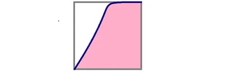
- In banking scoring, AUC_ROC is a very popular functionality, although it’s obvious that it’s not very suitable here either. The bank can issue a limited number of loans, so the main requirement for the algorithm is that among the objects that received the lowest marks there are only representatives of class 0 (“will return the loaned money” if we believe that class 1 “will not return the loaned money” and the algorithm estimates the probability of the non-return). This can be judged by the shape of the ROC curve (as in fig. 10 below).