
Let’s discuss the highlights of the recent speech separation and recognition challenge as well as some tricks used by the winners.
The article was originally published on Towards Data Science.
About the competition
Not so long ago, there was a challenge for speech separation and recognition called CHIME-6. CHIME competitions have been held since 2011. The main distinguishing feature of these competitions is that conversational speech recorded in everyday home environments on several devices simultaneously is used to train and evaluate participants’ solutions.
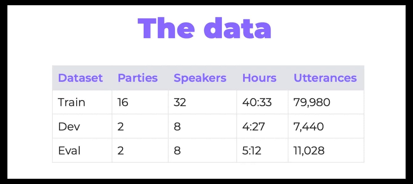
The data provided for the competition was recorded during the “home parties” of the four participants. These parties were recorded on 32 channels at the same time (six four-channel Microsoft Kinects in the room + two-channel microphones on each of the four speakers).
There were 20 parties, all of them lasting 2–3 hours. The organizers have chosen some of them for testing:
By the way, it was the same dataset that had been used in the previous CHIME-5 challenge. However, the organizers prepared several techniques to improve data quality (see the description of software baselines on GitHub, sections “Array synchronization” and “Speech enhancement”).
To find out more about the competition and data preparation here, visit its GitHub page or read the overview on Arxiv.org.
This year there were two tracks:
Track 1 — multiple-array speech recognition; Track 2 — multiple-array diarization and recognition.
And for each track, there were two separate ranking categories:
Ranking A — systems based on conventional acoustic modeling and official language modeling;
Ranking B — all other systems, including systems based on the end-to-end ASR baseline or systems whose lexicon and/or language model have been modified.
The organizers provided a baseline for participation, which includes a pipeline based on the Kaldi speech recognition toolkit.
The main criterion for evaluating participants was the speech recognition metric — word error rate (WER). For the second track, two additional metrics were used — diarization error rate (DER) and Jaccard error rate (JER), which allow to evaluate the quality of the diarization task:
In the tables below, you can see the competition results:
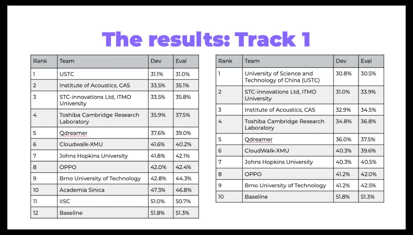
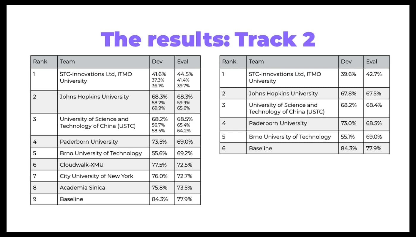
You can access the links to the papers on GitHub.
Here are a few curious things I’d like to discuss about the challenge: don’t want you to miss anything!
Challenge highlights
Research-oriented participation
In the previous CHiME-5 challenge, the Paderborn University team, who ranked 4th in Track 2, focused on a speech enhancement technique called Guided Source Separation (GSS). The results of the CHiME-5 competition have demonstrated that the technique improves other solutions.
This year, the organizers officially referred to GSS in the sound improvement section and included this technique in the baseline of the first track.
That is why many participants, including all the front runners, used GSS or a similar modification inspired by this idea.
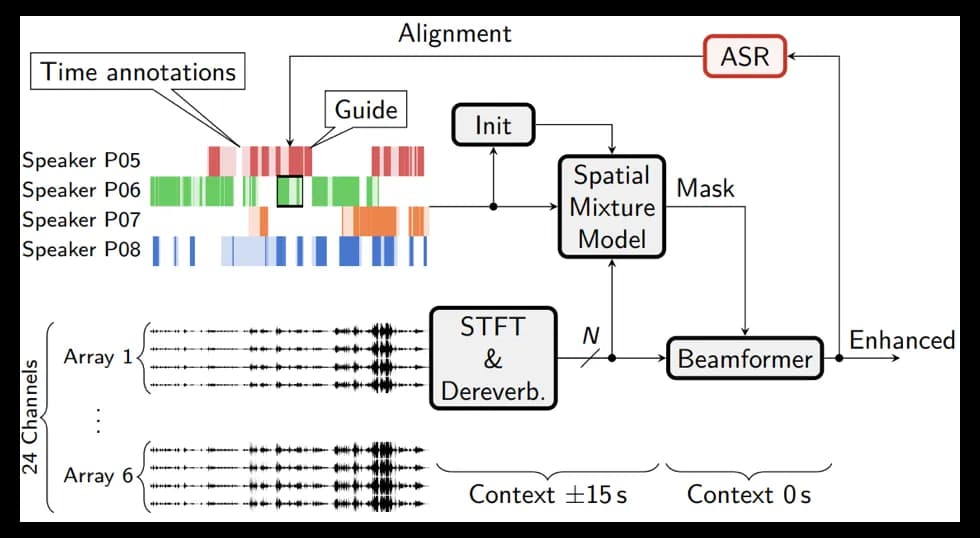
Here is how it works: you need to construct a Spatial Mixture Model (SMM), which allows to determine time-frequency masks for speakers (i.e., on what frequencies and at what time a given speaker was speaking). Training is performed using the EM algorithm with temporary annotations of speakers as initialization.
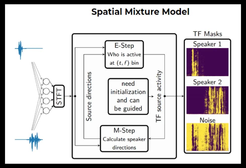
Then, this block is integrated into the general speech enhancement pipeline. This pipeline includes the dereverberation technique (i.e., removing the echo effect from a signal, which occurs when sound is reflected from the walls) and beamforming (i.e., generating a single signal from several audio tracks).
Since there were no speaker annotations for the second track, speech recognition alignments (time stamps of spoken phrases) were used to initialize the EM algorithm for training SMM.
You can read more about the technique and its implementation results in the Hitachi and Paderborn University team’s paper on Arxiv or take a look at their slides.
Solution for themselves
The USTC team, who ranked 1st in Track 1 and 3rd in Track 2, improved the solution they presented at the CHIME-5 challenge. This is the same team that won the CHIME-5 contest. However, other participants did not use the techniques described in their solution.
Inspired by the idea of GSS, USTC implemented its modification of the speech enhancement algorithm — IBF-SS.
You can find out more in their paper.
Baseline improvement
There were several evident weaknesses in the baseline that the organizers did not bother to hide: for example, using only one audio channel to build diarization or the lack of rescoring by the language model for ranking B. In baseline scripts, you can also find tips for improvement (for example, to add augmentation with noise from the CHIME-6 data to build x-vectors).
The JHU team solution completely eliminates all these weaknesses: there no brand new super efficient techniques, but the participants went over all the problem areas of the baseline. In Track 2, they ranked 2nd.
They explored multi-array processing techniques at each stage of the pipeline, such as multi-array GSS for enhancement, posterior fusion for speech activity detection, PLDA score fusion for diarization, and lattice combination for ASR. The GSS technique was described above. A good enough fusion technique, according to the JHU research, is simple max function.
Besides, they integrated techniques such as online multi-channel WPE dereverberation and VB-HMM based overlap assignment to deal with challenges like background noise and overlapping speakers, respectively.
More detailed description of the JHU solution can be found in their paper.
Track 2 winners: interesting tricks
I‘d like to highlight a few tricks that were used by the winners of the second track of the competition, the ITMO (STC) team:
WRN x-vectors
X-Vector is a speaker embedding, i.e a vector that contains speaker information. Such vectors are used in speaker recognition tasks. WRN x-vectors is an improvement of x-vectors through using the ResNet architecture and some other tricks. It has reduced DER so much that this technique alone would have been enough for the team to win the competition.
You can read more about WRN x-vectors in the paper by the ITMO team.
Cosine similarities and spectral clustering with automatic selection of the binarization threshold
By default, the Kaldi diarization pipeline includes extracting x-vectors from audio, calculating PLDA scores and clustering audio using agglomerative hierarchical clustering (AHC).
Now look at the PLDA component that used to build distances between speaker vectors. PLDA has a mathematical justification in calculating distances for I-Vectors. Put simply, it relies on the fact that I-Vectors contain information about the speaker and the channel, and when clustering, the only important thing for us is the speaker information. It also works nicely for X-Vectors.
However, using cosine similarity instead of PLDA scores and spectral clustering with automatic selection of a threshold instead of AHC allowed the ITMO team to make another significant improvement in diarization.
To find out more about spectral clustering with automatic selection of the binarization threshold, read this paper on Arxiv.org.
TS-VAD
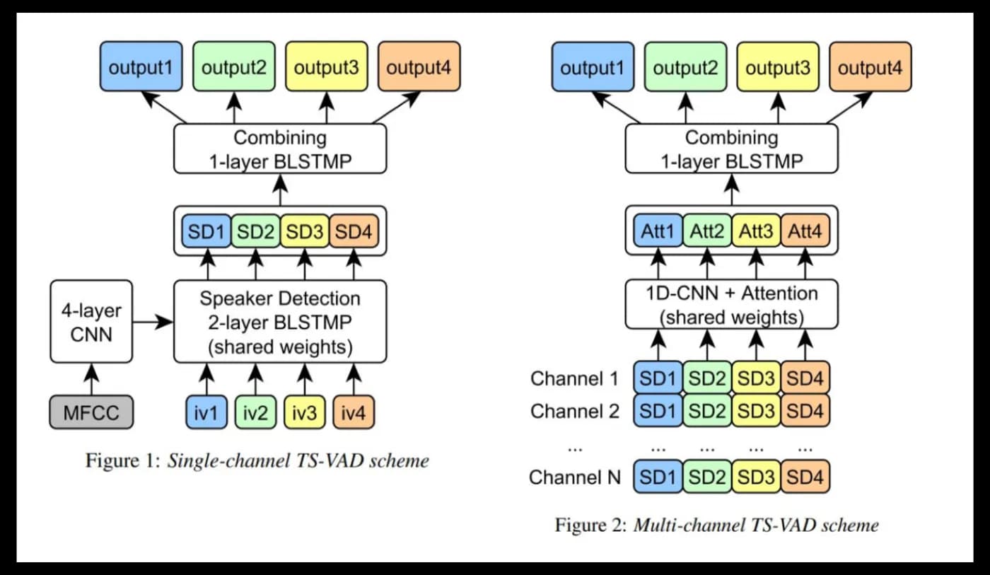
The authors focus specifically on this technique in their work. TS-VAD is a novel approach that predicts an activity of each speaker on each time frame. The TS-VAD model uses acoustic features (e.g., MFCC) along with i-vectors for each speaker as inputs. Two versions of TS-VAD are provided: single-channel and multi-channel. The architecture of this model is presented below.
Note that this network is tailored for dialogs of four participants, which is actually stipulated by the requirements of this challenge.
The single-channel TS-VAD model was designed to predict speech probabilities for all speakers simultaneously. This model with four output layers was trained using a sum of binary cross-entropies as a loss function. Authors also found that it is essential to process each speaker by the same Speaker Detection (SD) 2-layer BLSTMP, and then combine SD outputs for all speakers by one more BLSTMP layer.
The single-channel version of TS-VAD processes each channel separately. To process separate Kinect channels jointly, authors investigated the multi-channel TS-VAD model, which uses a combination of SD blocks outputs of the single TS-VAD model as an input. All the SD vectors for each speaker are passed through a 1-d convolutional layer and then combined by means of a simple attention mechanism. Combined outputs of attention for all speakers are passed through a single BLSTM layer and converted into a set of perframe probabilities of each speaker’s presence/absence.
Finally, to improve overall diarization performance, the ITMO team fused several single-channel and multi-channel TS-VAD models by computing a weighted average of their probability streams.
You can learn more about the TS-VAD model on Arxiv.org.
Conclusion
I hope this review has helped you get a better understanding of the CHiME-6 challenge. Maybe you’ll find the tips and tricks I mentioned useful if you decide to take part in the upcoming contests.
About the author: Dmitry is a machine learning researcher at Dasha.AI, a voice-first conversational platform. He specializes in speech technologies.