

Machine learning (ML) mainly answers such questions as “What?” / “Who?” / “How much?” as well as "What is depicted?" t and so on. The most natural human question that follows is “Why?”. In addition to the black box answer (whether it be boosting or a neural network), we would like to receive the argumentation of this answer. Below is an overview of the interpretation problem.
Why interpretations are necessary
There is no precise definition of the interpretation of the model for obvious reasons. However, we can all agree that the following problems lead to the necessity for interpretation:
One quality (model performance) metric (and even a set of metrics) does not describe the behavior of the model, but only the quality itself on a specific sample
The use of machine learning in “critical areas” (medicine, forensics, law, finance, politics, transport) gave rise to requirements for the security of the model, justification of confidence in it, as well as various procedures and documents regulating the use of ML-models
A natural requirement for an AI that is capable of answering the “What” question to justify the "Why" one. For example, children begin to ask this question even before they receive any in-depth knowledge. This is a natural stage in cognition: if you understand the logic of the process, then its effects and consequences become more obvious.
Interpretations are made for:
Explaining the results. As follows from the analysis of the problems above, this is the main purpose of interpretation
Improving the quality of the solution. If we understand how the model works, then options for improving it immediately appear. In addition, as we will see, some stages of interpretation, such as evaluating the importance of features, are used to solve ML problems (to form a feature space in particular)
Understanding how data works. There are a lot of caveats here, though: the model is interpreted, not the data! The model itself describes them with some error. Strictly speaking, data is not needed for interpretation; an already built (trained) model is needed
A check before implementation to make sure once again that nothing will break after the introduction of a black box into the business process.
What kinds of interpretations exist?
visualizations (images, diagrams, etc.)

For example, the figure above that I took from the Google AI Blog shows the synthesized images, which the network confidently classifies as "dumbbell". You can immediately see that a part of the hand is present in all the images. Apparently, there were no “no hands” in the images with dumbbells in the training sample. We identified this feature of the data without looking at the entire dataset!
tests

Fig. 2, taken from Hendricks, et al (2016), shows interesting examples of the so-called Visual Explanations, which are used when training a bunch of CNN + RNN to generate an explanation for a specific classification.
numbers, tables
Here is an example of the importance of features (see below).
object (s) / characteristics / data pieces
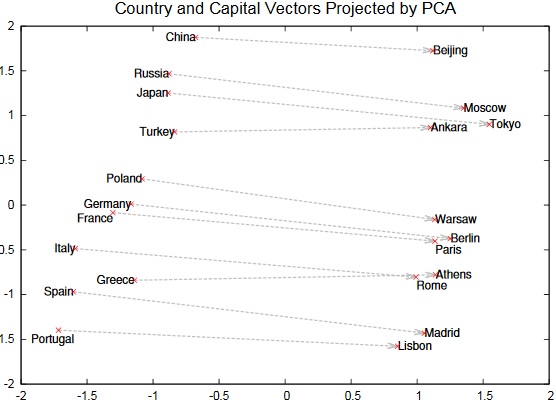
Fig. 3 shows the projections of words encodings (names of capitals and countries) of the word2vec method onto the two-dimensional subspace of the principal components of the 1000-dimensional encoding space. It can be seen that the first component distinguishes between the concepts (capital and country), while according to the second, the capitals and the corresponding countries seem to be ordered. Such patterns in the encoding space give credibility to the method.
Another example when the interpretation is carried out using parts of the generated object is shown in fig. 4 (Xu, et al (2016)). The problem of generating a description from an image is solved; for this, a bunch of CNN + RNN is also used. Which part of the image most influenced the output of a particular word in the description phrase is visualized here. It is quite logical that when a “bird” was the output, the neural network “looked” at it, when “above” was the output, the neural network looked under the bird, and when “water” was the output, it looked at the water.

analytical formula / simple model
Ideally, the model is written as a simple formula like this:

This is a linear model and it is not without reason that it is called interpreted. Each coefficient has a specific meaning here. For example, we can say that according to the model, an increase in the area of an apartment by 1 square foot increases its value by $200. Simple enough! Note that for logistic regression there is no such direct relationship with the answer, there is a relationship with the log likelihood…
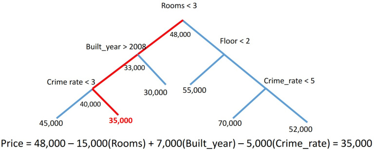
Formula interpretation is used for decision trees, random forests, and boosting. A separate prediction of these "monsters" can be easily written as a sum with weights similar to the above (however, it can contain a significant number of terms). This approach is implemented in the treeinterpreter library (sometimes called Saabas after the author of the library from Microsoft). The essence (for one tree) is shown in fig. 5. A specific forecast of a tree can be written as the sum of the bias (average of the target feature) and the sum over all branches of the changes in the average target feature in the subtree when passing through these branches. If we mark the terms with the features that correspond to the branches, add the terms with the same marks, then we get how much each feature “rejected” the tree response from the mean when generating a specific response.
Further we will discuss the approach when the black box is approximated by a simple interpreted model, usually by a linear one.
Interpretations can also be:
global (the operation of the model is described),
local (explains the specific answer of the model).
Requirements for interpretations
If we treat interpretations as explanations of work (and specific AI solutions), then this imposes the following requirements on them (for more details take a look at Explanation in Artificial Intelligence: Insights from the Social Sciences):
Interpretations should be contrastive. If a person was denied a loan, then he or she is not so much worried about the “why wasn’t I issued a loan?” as much as about the “why wasn’t I issued a loan, yet that guy was?” or "what am I missing to be issued a loan?"
Brevity and specificity (selectivity). Using the example of the same loan: it is strange to list a hundred reasons (even if the model uses 100 features), listing 1-3 of the most significant ones is highly desirable.
Specificity to content (taking customer focus into account). The explanation of the model's behavior should be client-oriented: take into account his language, subject area, etc.
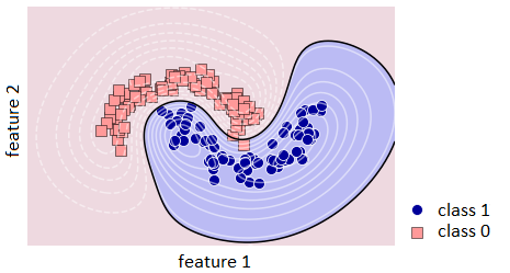
Meeting expectations and being truthful. It is strange to hear that you have not been issued a loan because your income is too high. Although some models, for example, SVM with kernels, can consider areas not covered by data to belong to arbitrary classes (this is a specificity of the geometry of the dividing surfaces, see the lower right corner in fig. 6). This is the key point! Some models are called uninterpretable not because of formal or analytical complexity, but, for example, because of the described features (non-monotonic result for monotonic data).
Truthfulness means that the explanation of the model must be true (no counterexample can be given to it).
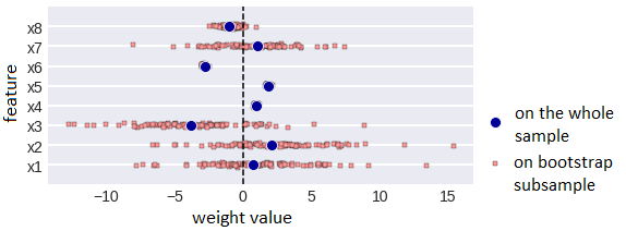
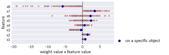
We’ve already said that the interpretation of linear regression coefficients satisfies all the requirements. They can also be depicted (as shown in fig. 7). 8 features are shown on the y-axis, the x-axis corresponds to the values of features when setting up the model on bootstrap subsamples (the stability of the weights is immediately visible), blue dots are the weights of the model trained on the entire sample.
It’s obvious that due to the different scales of trait it’s better to look not at weights, but at the effects of traits. Effect on a specific object of a specific feature is the product of the feature value by the weight value. Fugure 8 shows the effects of features in linear regression and you can select the effects of features for a specific object, in total they give the value of the regression on it. For clarity, you can use a box with a mustache (box-plot) or density plots.
Interpreting black boxes
1. Partial Dependence Analysis
Our black box depends on n features, in order to investigate the dependence on specific features, we need to integrate over the rest. It’s better to integrate to a measure that is consistent with the distribution of the data, so in practice it’s often done like this:
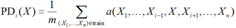
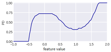
(so, we still use data here). This is a formula for dependence on a specific feature, it’s clear that the independence of features is assumed. For example, for the SVM model, the result of which is shown in fig. 5, a PDP (Partial Dependence Plot) is shown in fig. 9.
The research paper “Predicting pneumonia risk and hospital 30-day readmission” presents an analysis using such graphs, including the two-dimensional ones.
Analysis of the dependence of a pair of features is often done using H-statistics (Fridman and Popescu):
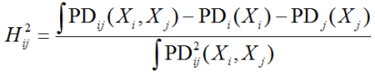
Integration here is the summation over all the elements of the sample. Such statistics describe how much the interaction of features brings to the model, but in reality, it takes quite a long time to calculate.
2. Individual Conditional Expectation
Partial dependence is too aggregated information, you can see how the response of the model on each object changes when a specific feature is varied. For our model example, such graphs are shown in fig. 10. A graph for one of the objects is highlighted in blue. The functions in question are often called Individual Conditional Expectation (ICE), it is clear that the arithmetic mean of ICE over all objects gives PD.

3. Feature Importance
One of the possibilities to analyze a model is to assess how much its solution depends on individual features. Many models appreciate the so-called Feature Importance. The simplest idea of assessing importance is to measure how quality deteriorates if the values of a particular attribute are spoiled. They usually spoil by mixing values (if the data is written in the matrix object-attribute, it is enough to make a random permutation of a specific column), since
it does not change the distribution for a specific trait,
this makes it possible not to train the model anew - the trained model is tested on a deferred sample with a damaged feature.
The method for assessing the importance of the features above is simple and has many remarkable properties, for example, the so-called consistency (if the model is changed so that it more significantly begins to depend on some feature, then its importance does not diminish). Many others, including the treeinterpreter described above, don’t have it.
Many people use the “feature_importances_” importance estimation methods built into the algorithms for constructing ensembles of trees. As a rule, they are based on calculating the total decrease in the minimized error functional using branching according to the considered feature. You need to note the following:
it’s not the importance of the feature for solving the problem, but only for setting up a specific model,
it’s easy to construct examples of the "exclusive OR" type, in which out of two identical features, the one that is used at the lower levels of the tree is of great importance (you can take a look at the explanation here),
these methods are inconsistent!
Interestingly, there are blog posts and articles comparing random forest implementations across different environments. At the same time, they try to use identical parameters, in particular, they include calculations of importance. None of the authors of such comparisons have demonstrated an understanding that the importance is calculated differently in different implementations, for example, in R/randomForest they use value shuffling, and in sklearn.ensemble.RandomForestClassifier they do it as we described above. It’s clear that the latest implementation will be much faster (and the point is not in the programming language, but in the complexity of the algorithm).
A non-trivial consensus method is the method implemented in the SHAP (SHapley Additive exPlanations) library. The importance of the i-th feature is calculated here by the following formula:
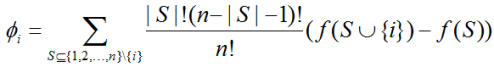
f(S) here is the response of the model trained on the set S of the set of n features (on a specific object - the whole formula is written for a specific object). It can be seen that the calculation requires retraining the model on all possible subsets of features, therefore, in practice, approximations of the formula are used, for example, using the Monte Carlo method.
Assessing the importance of features is a separate large topic that deserves a separate post, the most important thing is to understand the following:
there is no ideal algorithm for evaluating the importance of features (for any one can find an example when it does not work well),
if there are many similar (for example, strongly correlated features), then the importance can be "divided between them", therefore it is not recommended to drop features according to the importance threshold,
there is an old recommendation (however, without theoretical justification): the model for solving the problem and the assessment of importance should be based on different paradigms (for example, it is not recommended to evaluate the importance using RF and then tune it on important features).
4. Global Surrogate Models
We train a simple interpreted model that models the behavior of a black box. Note that it is not necessary to have data to train it (you can find out the responses of the black box on random objects and thus collect a training sample for the surrogate model).
The obvious problem here is that a simple model may not model the behavior of a complex one very well. They use various techniques for better tuning, some can be learned from the following paper: "Interpreting Deep Classifiers by Visual Distillation of Dark Knowledge". In particular, when interpreting neural networks, it’s necessary to not only use the class predicted by the network, but also all the probabilities of belonging to the classes that it received, the so-called Dark Knowledge.
5. Local Surrogate Models
Even if a simple model cannot simulate a complex one in the entire space, it is quite possible in the vicinity of a specific point. Local models explain a specific black box response. This idea is shown in Fig. 11. We have a black box built on data. At some point, it gives an answer, so we generate a sample in the vicinity of this point, find out the black box answers and set up an ordinary linear classifier. It describes a black box in the vicinity of a point, although throughout space it is very different from a black box. Fig. 11 shows the advantages and disadvantages of this approach are clear.

The popular interpreter LIME (Local Interpretable Model-agnostic, there is also an implementation in the eli5 library) is based on the described idea. As an illustration of its application fig. 12 shows the superpixels responsible for the high class probabilities in image classification (superpixel segmentation is performed first).
6. Exploring individual blocks of the mode
If the model naturally divides into blocks, you can interpret each block separately. In neural networks, they investigate which inputs cause the maximum activation of a particular neuron / channel / layer, as in fig. 13, which is taken from the distill.pub blog. These illustrations are much nicer than Fig. 1, since various regularizers were used in their creation, the ideas of which are as follows:
neighboring pixels of the generated image should not differ much,
the image is periodically "blurred" during generation,
we require image stability to some transformations,
we set the prior distribution on the generated images,
we do gradient descent not in the original, but in the so-called decorrelated space
For details check distill.pub.

Interpretations by example
1. Counterfactual explanations
Counterfactual explanations are objects that differ slightly, while the model's response to them differs significantly, as shown in fig. 14. Naturally, these may not be objects of the training sample. A search for a specific object of a conflicting pair will allow you to answer a question like "what needs to be done to be issued a loan?" It’s clear from fig. 14 that the geometry of such examples is clear (we are looking for a point/points near the surface separating the classes). The work "Explaining Data-Driven Document Classifications" provides a specific example of an explanation using conflicting examples in one text classification problem: "If words (welcome, fiction, erotic, enter, bdsm, adult) are removed, then class changes for adult to non-adult".FIGURE 14
To find conflicting examples, they solve optimization problems like this:
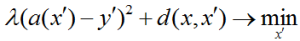
that is, they require a certain response of the model at the desired point and its small distance to a fixed one. There is also a special Growing Spheres method.
In the work "Anchors: High-precision model-agnostic explanations" considered, in a certain sense, the opposite concept - not what confuses and interferes with the correct classification, but what, on the contrary, forces the object to be classified in a certain way, the so-called Anchors, as seen in fig. 15.

A related concept to conflict examples of the so-called. examples of network attacks / Adversarial Examples. The difference is perhaps only in context. The former is used to explain the work of the black box, the latter to deliberately deceive it (incorrect work on "obvious" objects).
2. Influential Instances
Influential Instances are training set objects, on which the parameters of the tuned model depend heavily. For example, it is obvious that for the SVM method these are pivots. Also, anomalous objects are often influential objects. Fig. 16 shows a sample in which there is one outlier point, the linear regression coefficients will change significantly after removing only one of these objects from the sample, removing the rest of the objects does not change the model much.

It’s clear that the most natural algorithm for finding influential objects is enumerating objects and setting up a model on a sample without enumerating, but there are also tricky methods that do without enumeration using the so-called Influence Function.
3. Prototypes and Criticisms
Prototypes (or standards, or typical objects) are objects of the sample, which together describe it well, for example, are the centers of clusters if the objects form a cluster structure.
Criticism is objects that are very different from prototypes. Anomalies are criticism, but quite typical objects can also be criticism due to the wrong choice of a set of prototypes, as in fig. 17.

It’s clear that criticism and prototypes are needed to interpret the data, not the model, but they are useful because they can be used to understand what difficulties the model may face when setting up and on which examples it is better to test its operation. For example, in “Examples are not Enough, Learn to Criticize! Criticism for Interpretability” provides the following examples, as in fig. 18: depictions of certain dog breeds, which are very different from others, are inherent: unnatural animal postures, a large number of subjects, costumes on animals, etc. All this can reduce the effectiveness of determining the breed from a photograph.
