

Let’s talk about self-supervised machine learning - a way to teach a model a lot without manual markup, as well as an opportunity to avoid deep learning when setting a model up to solve a problem. This material requires an intermediate level of preparation; there are many references to original publications.
There are the following types of learning:
(Supervised Learning / SL: It’s training using labeled data where the training set consists of pairs (x, y), where x is the description of the object, y is its label, and where it is necessary to train the y = f (x) model, which is labeled according to descriptions.
Semi-Supervised Learning / SS: It’s training with partially labeled data, where the training set consists of data with and without labels (the latter, as a rule, is much larger). It is also necessary to train the y = f (x) model. Additional information on the way the objects are arranged could be of help here (see fig. 1). A text document classifier is a common semi-supervised machine learning example. The algorithm can learn from a few labeled documents and make predictions to classify a large volume of unlabeled text. Self-training machine learning is a technique in semi-supervised learning. On a conceptual level, self-training machine learning entails retraining the algorithm using labeled data and pseudo-labels generated after it classifies unlabeled data.
![fig 1]()
fig 1 Unsupervised Learning / UL: It’s training using unlabeled data, where only the unlabeled objects are given. It is necessary to effectively describe how the objects are positioned in the description space. For example, the typical untagged data learning tasks such as clustering, dimensionality reduction, anomaly detection, density estimation, etc. So, what’s the difference between supervised and unsupervised machine learning with an example? Unsupervised learning doesn’t need labeled data, hence its use in anomaly detection, clustering, etc. Supervised learning requires training with labeled data, and its main application is image recognition.

Let’s skip the description of Reinforcement Learning, which is the basic type of training, and go straight to the description of Self-Supervised Learning (SSL) that has become popular in recent years. So, what is self-supervised learning? It’s regarded as a subclass of unsupervised learning as it entails working with data without manually added labels.
There is a huge unlabeled sample here, it is necessary to form a pseudo label for each object and solve the resulting SL-problem, yet we are not so much interested in the quality of the solution to the problem we invented (so-called pretext task), but in the representation of objects, which will be learned in the course of solving it. This representation can be used in the future when solving SL tasks, also known as downstream tasks.
One of the main reasons for self-supervised machine learning is a small amount of labeled data (in this case, there is a temptation to use unlabeled data, possibly from a different domain). Unlike training with partially labeled data, SSL uses completely arbitrary unlabeled data that is not related to the problem being solved.
Let's look at some self-supervised learning examples, and then get back to its definition. Around 80% of modern word processing (NLP) consists of SSL. With the help of SSL, almost all representations of words and texts are obtained. For instance, in the classical word2vec algorithm, you take an unlabeled text corpus followed by coming up with a problem with labels (a supervised machine learning example would be taking neighboring words to predict the central word or, conversely, taking the central word to predict those adjacent to it). Then, a simple neural network is trained on this problem, getting representations of words (and weights of the trained network), which are already used in other tasks, unrelated to the pretext task. This approach is often called transfer learning. Generally speaking, transfer learning is a broad concept and refers to using a model that’s been trained to solve problem ”a” to solve problem “b”. In self-supervised learning, it is important that the markup in pseudo-marks is obtained automatically. For example, representations obtained by the Cove method, which uses an encoder for a machine translation task, would be transferred, not self-supervised.
Let's get back to the definition of self-supervised machine learning and go over some terms:
A pretext task is a task with artificially created labels (pseudo-labels), on which the model is trained to learn good representations of objects. For example, there is hope that in the neural network the initial and middle layers will be first trained on the pretext task, frozen later on in order to then train the last layers.
Pseudo-labels are labels that are obtained automatically, without any manual labeling, and teaching of such contributes to the formation of good representations.
Downstream task is a task that evaluates the quality of features learned by self supervised learning. In almost all experiments in self-supervised learning articles, simple models are trained on the received feature representations in downstream tasks: logistic regression or the nearest neighbor method. Thus, self-supervised machine learning is a direction in deep learning that seeks to make deep learning a data preprocessing procedure. As such, networks are needed to form features, are trained on cheap markup of large sets of initially unlabeled data, and the problem itself is solved by a simple model.
Let's talk about the history of the development of SSL and use image processing as an example. At the first stage of development of this area, experiments were carried out mainly with the formulation of downstream tasks. The main goal here was to figure out how to automatically add labels so that self-supervised models get good representations. For example, in convolutional neural networks for image processing, the first and middle layers were trained, which are known to be responsible for detecting edges, corners, and some kind of abstract forms.
1. Predicting (spatial) context
Let’s take a look at the following self-supervised learning tutorial. A random patch is selected - in this case, it is a rectangular area of the image with eight adjacent patches (see fig. 2) and one of them is selected. Naturally, by looking at paired patches ("central patch", "neighboring"), a person can easily determine how the adjacent one is located relative to the central one. If a neural network learns to detect this, then it understands how the objects of the real world are arranged (the wheels of the truck are lower than the cab, and the hat of a person is higher than the face, etc.). It seems intuitive that when the network learns this task, then its lower layers must learn to perfectly detect edges, corners, etc.
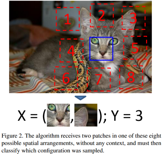
fig. 2, publication [2] [2] Doersch, A. Gupta, and A. A. Efros. Unsupervised visual representation learning by context prediction. In International Conference on Computer Vision (ICCV), 2015
There are several "hacks" in the implementation of the method which will be described here since they are often used in self-supervised machine learning. In fig. 2 it can be seen that the patches are located with a gap and random displacement. This is done to complicate the task because a person can assemble a puzzle from pieces without thinking about the meaning of what is depicted (by looking at how the puzzle joints are coordinated), but we would want the neural network to "understand" that is shown, not to find similar joints. Another trick is that in such methods you can “spoil the colors”; in this example, for instance, two random channels were clogged with noise. This is due to the laws of optics (chromatic aberration): all modern images were taken using photo/video equipment and they have a shift in the difference in the average for RGB channels when moving from the center to the edges (for example, you can train a network that will quite accurately determine which part of the image the patch is cut from). To prevent the network from using this feature when solving a pretext task, the channels are spoiled.
2. Predicting image rotation
Another task that can be easily solved by a person, and the labels which are obtained automatically, is the task to determine the angle by which the image was rotated (fig. 3). The image is taken and rotated at a random angle and this angle is declared as a label of the resulting image. Experiments have shown that it is better to rotate by an angle multiple of 90 degrees and, thus, to solve a problem with 4 classes. It is notable that the network in the pretext task pays attention to where the head of the depicted person or animal is, or to where the eyes/mouth is, or whether the head is depicted too large. In essence, having come up with an artificial problem, we taught the network to detect the head without planning on doing so! Note that this technique does not work with all data (sometimes images do not have an objective correct orientation).
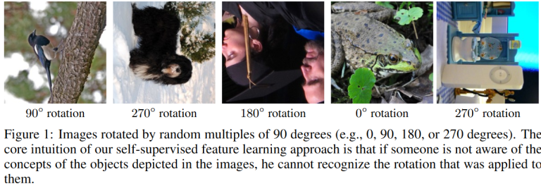
pic 3. [3] Gidaris, P. Singh, and N. Komodakis. Unsupervised representation learning by predicting image rotations. In International Conference on Learning Representations (ICLR), 2018.
3. Exemplar
This is the name of a group of methods that use image patches. In one of the first articles, “interesting fragments” were selected from the images, and then they were augmented. The task was to determine the number of the original image by looking at the augmented patch. Sometimes this is referred to as a method in which it needs to be determined whether a pair of patches were taken from the same image or from the different ones.
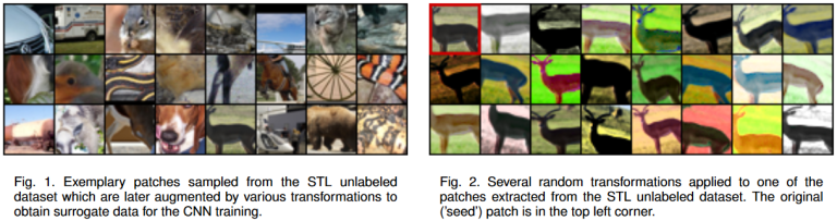
fig 4. [4] Dosovitskiy, J. T. Springenberg, M. Riedmiller, and T. Brox Discriminative unsupervised feature learning with convolutional neural networks. In Advances in Neural Information Processing Systems (NIPS), 2014.
4. Jigsaw puzzle
Fig. 5 shows the basic idea of the Jigsaw puzzle. You select one random patch and select the neighboring ones so that there is a total of 9 patches, then mix them. It is not difficult for a person to put them back in order. The neural network is required to do the same. According to the ordered list of patches, the neural network must determine the number of permutation that needs to be applied in order to put the patches back in order. The same tricks are applied here as in method number 1 (in addition to independent patch normalization).
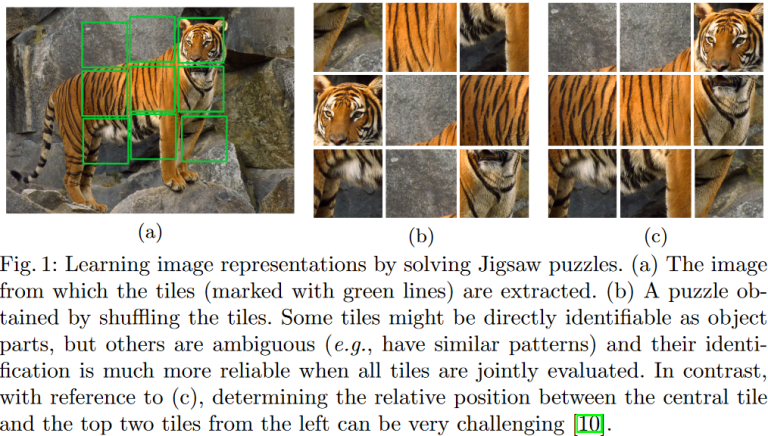
fig. 5 [5] Noroozi and P. Favaro. Unsupervised learning of visual representations by solving jigsaw puzzles. In European Conference on Computer Vision (ECCV), 2016.
There are various generalizations of the described method. An example of that would be mixing "extra" patches (taken from another image) into the puzzle. Or, as shown in fig. 6, a very ambitious pretext task is posed, which is to complete the discolored damaged puzzle, color its elements, and draw the missing fragment.
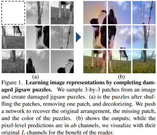
fig. 6 [6] Kim, D., Cho, D., Yoo, D., and Kweon, I. S. Learning Image Representations by Completing Damaged Jigsaw Puzzles. In WACV 2018, 2018.
5. DeepCluster
It is known that if you accidentally initialize AlexNet and adjust the weights of only the last layer (that is, solving the problem with factual logistic regression), then the quality on ImageNet will be 12% (recall that there are 1000 classes in the problem), so even a random network generates a good feature space. In the DeepCluster method, k-means-clustering is done in this space, the cluster numbers are declared as labels and the network is trained for the resulting SL-classification problem, then the procedure is repeated - we cluster again and take several training steps. It has been established that overclustering is good to be used in this approach - the number of clusters should be quite large. For example, for self-supervised learning on ImageNet, the "objective classes" numbers are 10 times larger.
[7] Caron, P. Bojanowski, A. Joulin, and M. Douze. Deep clustering for unsupervised learning of visual features. European Conference on Computer Vision (ECCV), 2018.
6. Context Encoder
A patch (or even an area of arbitrary shape) is removed from an image and a neural network is trained to restore it. On fig. 7 you can see that a human artist coped well with this task.
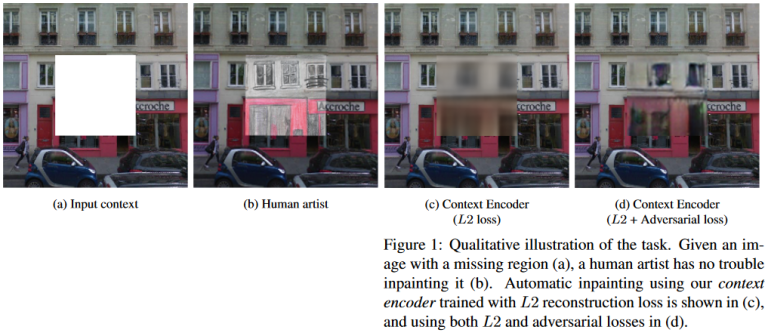
fig 7. [8] Pathak, P. Krahenbuhl, J. Donahue, T. Darrell, and A. Efros. Context encoders: Feature learning by inpainting. In Conference on Computer Vision and Pattern Recognition (CVPR), 2016.
7. Channel restoration
As a pretext task, you can choose the coloring of images. Take a collection of images, translate each one into grayscale, and, using the "discolored" image, teach the neural network to get a colored one. More precisely, restore the values of the a, b channels in CIELAB encoding.[9] Zhang, P. Isola, and A. A. Efros. Colorful image colorization. In European Conference on Computer Vision (ECCV), 2016.
In a more advanced version, you can train a split-brain autoencoder, which uses one channel to restore the other ones and vice versa.
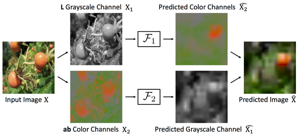
fig.8 [10] Zhang, P. Isola, and A. A. Efros. Split-brain autoencoders: Unsupervised learning by cross-channel prediction. In Conference on Computer Vision and Pattern Recognition(CVPR), 2017
8. Video markup
If we have a collection of video clips, then there is a larger scope for setting pretext tasks. For example, you can take two adjacent frames and use the first one to teach the neural network to determine what pixels will change their position on the second frame (fig. 9). Usually, objects move on the video as a whole, which allows the network to immediately learn how to solve the segmentation problem without the necessity of manual marking. In practice, this automatic layout is very noisy (fig. 9), but in the end, it allows you to teach the network to find objects in images.
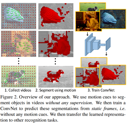
fig. 9 [11] Pathak, R. B. Girshick, P. Dollar, T. Darrell, and B. Hariharan. Learning features by watching objects move. In Conference on Computer Vision and Pattern Recognition(CVPR), 2017.
Another interesting approach to the formulation of the pretext task was proposed in [12]. We take two sequential frames, desaturate the second, train the neural network to paint it according to the colored one, and then the decolorized one. The coloring happens as follows: the CNN network generates descriptions of the location. Then, the network uses the color that matches the colored image location most, then it colors the decolorized image; i.e. the network actually learns to match pixels on two consecutive frames.
[12] Carl Vondrick, Abhinav Shrivastava, Alireza Fathi, Sergio Guadarrama, Kevin Murphy «Tracking Emerges by Colorizing Videos»
9. Counting visual primitives
Let's say we are counting something in images, for example, eyes. If we split the image into parts, then the sum of the number of eyes in those parts would be equal to the number of eyes in the entire image, and if we take a random image, then, most likely, it will have a different number of eyes. These ideas are embedded in the network architecture shown in fig. 10, it is this architecture that is being taught in the pretext test.
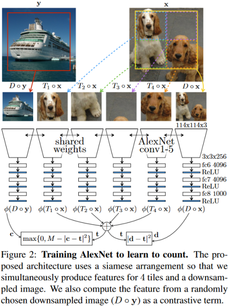
fig 10. [13] Noroozi, H. Pirsiavash, and P. Favaro. Representation learning by learning to count. In International Conferenceon Computer Vision (ICCV), 2017.
10. Self-study ensembles
In the article [14], several pretext tasks are solved at once. To be more precise, one neural network with several output heads is trained, and each of those solves one of the pretext tasks. As in other areas of machine learning, ensembles are superior to their individual components.
[14] Carl Doersch, Andrew Zisserman «Multi-task Self-Supervised Visual Learning»
Contemporary self-supervised learning trends
In recent years, much fewer papers were published on the selection of pretext tasks, since the main direction in self-supervised learning has become what’s called Contrastive Learning. A pair of objects is placed to the input of the neural network and it determines whether they are similar or not. An augmented patch from an image is served as an object. The patches from one image should be similar, and the patches from different images should be different. Mutual information or related functions are used as optimized functions, for example, the InfoNCE lower bound:
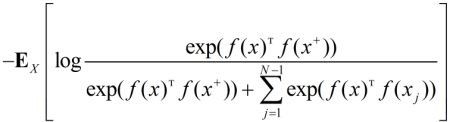
x refers to the selected patch, called the anchor, x+ refers a patch similar to x, xj refers to a patch different from x (there are N-1 of them), f () refers to the object's encoder (representing it as a real vector). This error function almost turns into a Triplet Loss if you only use one negative example.
Modern methods fall under the following scheme:
Invariant Information Clustering (IIC) - mutual information is optimized, a network that performs soft classification is used.
[15] Ji, J. F. Henriques, and A. Vedaldi. Invariant information clustering for unsupervised image classification and segmentation. In Proceedings of the IEEE International Conference on Computer Vision, pages 9865–9874, 2019.
Deep InfoMax (DIM) is optimized by MI between the input of the neural network (where we place the image) and the learned high-level representation and can be implemented in different ways (for example via InfoNCE). To make the representation satisfy certain statistical properties, adversarial learning is used. In addition, representations of individual image patches are obtained (they form an N × N grid), which are concatenated with the global representation to optimize InfoNCE.
[16] D. Hjelm, A. Fedorov, S. Lavoie-Marchildon,K. Grewal, P. Bachman, A. Trischler, and Y. Bengio. Learning deep representations by mutual information estimation and maximization. In International Conference on Learning Representations, 2019.
Augmented Multiscale Deep InfoMax (AMDIM)
An advanced implementation of the previous approach.
[17] Bachman, R. D. Hjelm, and W. Buchwalter. Learning representations by maximizing mutual information across views. In Advances in Neural Information Processing Systems, p. 15509–15519, 2019.
Contrastive Predictive Coding (CPC)
This approach is summarized into different data formats, Fig. 11 shows its application to audio data. We train the encoder, which turns the audio fragment into a description zt, and then the description is submitted into a recurrent network that predicts the descriptions of the following fragments. Again, InfoNCE-loss is optimized here - the forecast should look like a continuation and different from randomly taken audio fragments. Similarly, CPC is applied to images that are divided into a grid of 49 patches (7 × 7) according to the description of the upper part of the image, we predict the descriptions of the lower one. CPC is also used for textual data and in reinforcement learning (where we try to predict a description of the state of the environment, while CPC is an additional penalty to the main one).

fig 11. [18] v. d. Oord, Y. Li, and O. Vinyals. Representation learning with contrastive predictive coding
There is the latest implementation of the method from [18b], in which many experiments were done (with architectures, methods of normalization, etc.), as a result, the quality of self-supervised learning surpassed the quality of conventional training using labeled data on ImageNet (96.5% Top-5 accuracy versus 95.2 %).
[18b] Olivier J. Henaff, Ali Razavi, Carl Doersch, S. M. Ali Eslami, Aaron van den Oord «Data-Efficient Image Recognition with Contrastive Predictive Coding»
Momentum Contrast (MoCo)
In comparative learning, the more negative examples the better. Usually, this number is limited by the size of the batch. The MoCo method maintains a dynamic queue of negative examples (when another batch of examples arrives, the oldest batch is removed from the queue). One of the tricks of the method is the way to update the encoder parameters (it takes too long to pass gradients through a large queue).
[19] Kaiming He, Haoqi Fan, Yuxin Wu, Saining Xie, Ross Girshick «Momentum Contrast for Unsupervised Visual Representation Learning»
There is a more up-to-date version of the algorithm that was published recently, it borrowed some tricks from the following approach.
[20] Xinlei Chen, Haoqi Fan, Ross Girshick, Kaiming He «Improved Baselines with Momentum Contrastive Learning»
SimCLR: A Simple Framework for Contrastive Learning of Visual Representations
This method was published a few months ago, and in fact, it is just a good library in which everything is correctly implemented: a standard comparative learning scheme and a ResNet-based encoder are taken, the representation is passed through a two-layer network to obtain vectors over which Contrastive loss is already measured (such network is exactly what brings the novelty). Experiments have been carried out with different augmentations. One of the features is effective implementation. For example, we take N images, from which we select 2 augmented patches, where each can act as an anchor, and it will have 1 positive and 2N-2 negative.
[21] Ting Chen, Simon Kornblith, Mohammad Norouzi, Geoffrey Hinton «A Simple Framework for Contrastive Learning of Visual Representations»
Applications
When coding categorical features, which are common in the description of customers and operations (MCC-transaction codes, profession, branch number, etc.), a technique similar to word2vec is successfully used.
It is great to use mask recovery on transactions, similarly to how it is done in BERT, the Transformer architecture is also suitable here (though it should not be applied head-on; for example, the positional coding of tokens for transactions is trickier than for words in a sentence, because each transaction has a specific time that it took place).
Self-supervised learning of the recurrent network works well on transactions with the pretext task such as whether “the correct order of transactions was inputted”.
Another trick that works in financial data is “using bad” data for self-supervised learning. The fact is that the distribution of indicators of characteristics of customer descriptions changes over time means it is impossible to train on all data - it is distributed differently than the data on which the algorithm will have to work. The sample for training is specially selected from all data, but the data that is not suitable for training can be useful for self-supervised learning.
A very cool technique for self-supervised learning is using the data of video cameras in offices, so to solve the problem with the markup defined by accompanying sound recordings. The idea can be viewed here. After such self-supervised learning, tasks such as detecting an emergency situation, large queues or scandals are solved using a small marked sample.
In this post, there are some very good techniques for self-supervised learning in business cases. For instance, the last one described can save a lot of time and allow you to solve a problem with a small markup, though it’s important to keep in mind that this technique was not described in detail, and in self-supervised learning, there are a lot of subtleties in the correctness of implementation (for example, the above mentioned technique of adding noise to RGB-channels).
Notable links
You can follow the progress in this area on paperswithcode (but only for image classification).
Some good overviews:
Schmarje L. et al. A survey on Semi-, Self-and Unsupervised Techniques in Image Classification
Longlong Jing and Yingli Tian «Self-supervised Visual Feature Learning with Deep Neural Networks: A Survey»
Guo-Jun Qi, Jiebo Luo «Small Data Challenges in Big Data Era: A Survey of Recent Progress on Unsupervised and Semi-Supervised Methods»
Collections of articles on this topic: